Recently, I gave a couple of perspective talks on quantum advantage, one at the annual retreat of the CIQC and one at a recent KITP programme. I started off by polling the audience on who believed quantum advantage had been achieved. Just this one, simple question.

The audience was mostly experimental and theoretical physicists with a few CS theory folks sprinkled in. I was sure that these audiences would be overwhelmingly convinced of the successful demonstration of quantum advantage. After all, more than half a decade has passed since the first experimental claim (G1) of “quantum supremacy” as the patron of this blog’s institute called the idea “to perform tasks with controlled quantum systems going beyond what can be achieved with ordinary digital computers” (Preskill, p. 2) back in 2012. Yes, this first experiment by the Google team may have been simulated in the meantime, but it was only the first in an impressive series of similar demonstrations that became bigger and better with every year that passed. Surely, so I thought, a significant part of my audiences would have been convinced of quantum advantage even before Google’s claim, when so-called quantum simulation experiments claimed to have performed computations that no classical computer could do (e.g. (qSim)).

I could not have been more wrong.

In both talks, less than half of the people in the audience thought that quantum advantage had been achieved.

In the discussions that ensued, I came to understand what folks criticized about the experiments that have been performed and even the concept of quantum advantage to begin with. But more on that later. Most of all, it seemed to me, the community had dismissed Google’s advantage claim because of the classical simulation shortly after. It hadn’t quite kept track of all the advances—theoretical and experimental—since then.

In a mini-series of three posts, I want to remedy this and convince you that the existing quantum computers can perform tasks that no classical computer can do. Let me caution, though, that the experiments I am going to talk about solve a (nearly) useless task. Nothing of what I say implies that you should (yet) be worried about your bank accounts.

I will start off by recapping what quantum advantage is and how it has been demonstrated in a set of experiments over the past few years.

Part 1: What is quantum advantage and what has been done?

To state the obvious: we are now fairly convinced that noiseless quantum computers would be able solve problems efficiently that no classical computer could solve. In fact, we have been convinced of that already since the mid-90ies when Lloyd and Shor discovered two basic quantum algorithms: simulating quantum systems and factoring large numbers. Both of these are tasks where we are as certain as we could be that no classical computer can solve them. So why talk about quantum advantage 20 and 30 years later?

The idea of a quantum advantage demonstration—be it on a completely useless task even—emerged as a milestone for the field in the 2010s. Achieving quantum advantage would finally demonstrate that quantum computing was not just a random idea of a bunch of academics who took quantum mechanics too seriously. It would show that quantum speedups are real: We can actually build quantum devices, control their states and the noise in them, and use them to solve tasks which not even the largest classical supercomputers could do—and these are very large.

What is quantum advantage?

But what exactly do we mean by “quantum advantage”. It is a vague concept, for sure. But some essential criteria that a demonstration should certainly satisfy are probably the following.

1. The quantum device needs to solve a pre-specified computational task. This means that there needs to be an input to the quantum computer. Given the input, the quantum computer must then be programmed to solve the task for the given input. This may sound trivial. But it is crucial because it delineates programmable computing devices from just experiments on any odd physical system.
2. There must be a scaling difference in the time it takes for a quantum computer to solve the task and the time it takes for a classical computer. As we make the problem or input size larger, the difference between the quantum and classical solution times should increase disproportionately, ideally exponentially.
3. And finally: the actual task solved by the quantum computer should not be solvable by any classical machine (at the time).

Achieving this last criterion using imperfect, noisy quantum devices is the challenge the idea of quantum supremacy set for the field. After all, running any of our favourite quantum algorithms in a classically hard regime on these devices is completely out of the question. They are too small and too noisy. So the field had to come up with the conceivably smallest and most noise-robust quantum algorithm that has a significant scaling advantage against classical computation.

Random circuits are really hard to simulate!

The idea is simple: we just run a random computation, constructed in a way that is as favorable as we can make it to the quantum device while being as hard as possible classically. This may strike as a pretty unfair way to come up with a computational task—it is just built to be hard for classical computers without any other purpose. But: it is a fine computational task. There is an input: the description of the quantum circuit, drawn randomly. The device needs to be programmed to run this exact circuit. And there is a task: just return whatever this quantum computation would return. These are strings of 0s and 1s drawn from a certain distribution. Getting the distribution of the strings right for a given input circuit is the computational task.

This task, dubbed random circuit sampling, can be solved on a classical as well as a quantum computer, but there is a (presumably) exponential advantage for the quantum computer. More on that in Part 2.

For now, let me tell you about the experimental demonstrations of random circuit sampling. Allow me to be slightly more formal. The task solved in random circuit sampling is to produce bit strings $x \in \{0,1\}^n$ distributed according to the Born-rule outcome distribution

$p_C(x) = | \bra x C \ket {0}|^2$

of a sequence of elementary quantum operations (unitary rotations of one or two qubits at a time) which is drawn randomly according to certain rules. This circuit $C$ is applied to a reference state $\ket 0$ on the quantum computer and then measured, giving the string $x$ as an outcome.

The breakthrough: classically hard programmable quantum computations in the real world

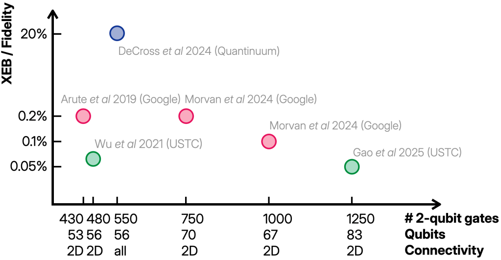
In the first quantum supremacy experiment (G1) by the Google team, the quantum computer was built from 53 superconducting qubits arranged in a 2D grid. The operations were randomly chosen simple one-qubit gates ($\sqrt X, \sqrt Y, \sqrt{X+Y}$) and deterministic two-qubit gates called fSim applied in the 2D pattern, and repeated a certain number of times (the depth of the circuit). The limiting factor in these experiments was the quality of the two-qubit gates and the measurements, with error probabilities around 0.6 % and 4 %, respectively.

A very similar experiment was performed by the USTC team on 56 qubits (U1) and both experiments were repeated with better fidelities (0.4 % and 1 % for two-qubit gates and measurements) and slightly larger system sizes (70 and 83 qubits, respectively) in the past two years (G2,U2).

Using a trapped-ion architecture, the Quantinuum team also demonstrated random circuit sampling on 56 qubits but with arbitrary connectivity (random regular graphs) (Q). There, the two-qubit gates were $\pi/2$-rotations around $Z \otimes Z$, the single-qubit gates were uniformly random and the error rates much better (0.15 % for both two-qubit gate and measurement errors).

All the experiments ran random circuits on varying system sizes and circuit depths, and collected thousands to millions of samples from a few random circuits at a given size. To benchmark the quality of the samples, the widely accepted benchmark is now the linear cross-entropy (XEB) benchmark defined as

$\chi = 2^n \mathbb E_C \mathbb E_{x} p_C(x) -1 ,$

for an $n$-qubit circuit. The expectation over $C$ is over the random choice of circuit and the expectation over $x$ is over the experimental distribution of the bit strings. In other words, to compute the XEB given a list of samples, you ‘just’ need to compute the ideal probability of obtaining that sample from the circuit $C$ and average the outcomes.

The XEB is nice because it gives 1 for ideal samples from sufficiently random circuits and 0 for uniformly random samples, and it can be estimated accurately from just a few samples. Under the right conditions, it turns out to be a good proxy for the many-body fidelity of the quantum state prepared just before the measurement.

This tells us that we should expect an XEB score of $(1-\text{error per gate})^{\text{\# gates}} \sim c^{- n d }$ for some noise- and architecture-dependent constant $c$. All of the experiments achieved a value of the XEB that was significantly (in the statistical sense) far away from 0 as you can see in the plot below. This shows that something nontrivial is going on in the experiments, because the fidelity we expect for a maximally mixed or random state is $2^{-n}$ which is less than $10^{-14}$ % for all the experiments.

The complexity of simulating these experiments is roughly governed by an exponential in either the number of qubits or the maximum bipartite entanglement generated. Figure 5 of the Quantinuum paper has a nice comparison.

It is not easy to say how much leverage an XEB significantly lower than 1 gives a classical spoofer. But one can certainly use it to judiciously change the circuit a tiny bit to make it easier to simulate.

Even then, reproducing the low scores between 0.05 % and 0.2 % of the experiments is extremely hard on classical computers. To the best of my knowledge, producing samples that match the experimental XEB score has only been achieved for the first experiment from 2019 (PCZ). This simulation already exploited the relatively low XEB score to simplify the computation, but even for the slightly larger 56 qubit experiments these techniques may not be feasibly run. So to the best of my knowledge, the only one of the experiments which may actually have been simulated is the 2019 experiment by the Google team.

If there are better methods, or computers, or more willingness to spend money on simulating random circuits today, though, I would be very excited to hear about it!

Proxy of a proxy of a benchmark

Now, you may be wondering: “How do you even compute the XEB or fidelity in a quantum advantage experiment in the first place? Doesn’t it require computing outcome probabilities of the supposedly hard quantum circuits?” And that is indeed a very good question. After all, the quantum advantage of random circuit sampling is based on the hardness of computing these probabilities. This is why, to get an estimate of the XEB in the advantage regime, the experiments needed to use proxies and extrapolation from classically tractable regimes.

This will be important for Part 2 of this series, where I will discuss the evidence we have for quantum advantage, so let me give you some more detail. To extrapolate, one can just run smaller circuits of increasing sizes and extrapolate to the size in the advantage regime. Alternatively, one can run circuits with the same number of gates but with added structure that makes them classically simulatable and extrapolate to the advantage circuits. Extrapolation is based on samples from different experiments from the quantum advantage experiments. All of the experiments did this.

A separate estimate of the XEB score is based on proxies. An XEB proxy uses the samples from the advantage experiments, but computes a different quantity than the XEB that can actually be computed and for which one can collect independent numerical and theoretical evidence that it matches the XEB in the relevant regime. For example, the Google experiments averaged outcome probabilities of modified circuits that were related to the true circuits but easier to simulate.

The Quantinuum experiment did something entirely different, which is to estimate the fidelity of the advantage experiment by inverting the circuit on the quantum computer and measuring the probability of coming back to the initial state.

All of the methods used to estimate the XEB of the quantum advantage experiments required some independent verification based on numerics on smaller sizes and induction to larger sizes, as well as theoretical arguments.

In the end, the advantage claims are thus based on a proxy of a proxy of the quantum fidelity. This is not to say that the advantage claims do not hold. In fact, I will argue in my next post that this is just the way science works. I will also tell you more about the evidence that the experiments I described here actually demonstrate quantum advantage and discuss some skeptical arguments.

---

Let me close this first post with a few notes.

In describing the quantum supremacy experiments, I focused on random circuit sampling which is run on programmable digital quantum computers. What I neglected to talk about is boson sampling and Gaussian boson sampling, which are run on photonic devices and have also been experimentally demonstrated. The reason for this is that I think random circuits are conceptually cleaner since they are run on processors that are in principle capable of running an arbitrary quantum computation while the photonic devices used in boson sampling are much more limited and bear more resemblance to analog simulators.

I want to continue my poll here, so feel free to write in the comments whether or not you believe that quantum advantage has been demonstrated (by these experiments) and if not, why.

References

[G1] Arute, F. et al. Quantum supremacy using a programmable superconducting processor. Nature 574, 505–510 (2019).

[Preskill] Preskill, J. Quantum computing and the entanglement frontier. arXiv:1203.5813 (2012).

[qSim] Choi, J. et al. Exploring the many-body localization transition in two dimensions. Science 352, 1547–1552 (2016). .

[U1] Wu, Y. et al. Strong Quantum Computational Advantage Using a Superconducting Quantum Processor. Phys. Rev. Lett. 127, 180501 (2021).

[G2] Morvan, A. et al. Phase transitions in random circuit sampling. Nature 634, 328–333 (2024).

[U2] Gao, D. et al. Establishing a New Benchmark in Quantum Computational Advantage with 105-qubit Zuchongzhi 3.0 Processor. Phys. Rev. Lett. 134, 090601 (2025).

[Q] DeCross, M. et al. Computational Power of Random Quantum Circuits in Arbitrary Geometries. Phys. Rev. X 15, 021052 (2025).

[PCZ] Pan, F., Chen, K. & Zhang, P. Solving the sampling problem of the Sycamore quantum circuits. Phys. Rev. Lett. 129, 090502 (2022).