Rudy Marcus was 91 years old when I took a course from him. His age was, arguably, not his most remarkable quality.
The course took place during the second spring of my PhD. I was completing not only the academic year, but also my course requirements. Why not, I figured, indulge in traditional statistical mechanics? Statistical mechanics neighbors, and partially overlaps with, thermodynamics. Modern approaches to statistical mechanics include fancy toolkits imparted in physics courses: the renormalization-group method; Ginzburg–Landau theory; and the latter theory’s successor, topological order. I craved a more traditional approach, as won’t surprise readers of this blog. So I ditched the physics course list and signed up for Chemistry 166.
Rudy didn’t disappoint. He began the course with a tradition passed down from a founder of thermodynamics: Boltzmann’s H theorem. The theorem amounts to the first argument ever published for the second law of thermodynamics: every (sufficiently large) closed, isolated system’s entropy increases or remains constant; it doesn’t decrease. Rederiving Boltzmann’s H theorem, I felt as I would while holding a lace collar worn by Queen Elizabeth I: as though I were touching history.
Rudy proceeded through more of the greatest hits in statistical mechanics. For instance, the Fokker–Planck and Langevin equations describe random processes. Examples include the subject of one of Einstein’s most famous papers: the motion of a pollen grain suspended in a liquid and buffeted by the liquid’s molecules. Chemistry 166 provided much of the bread and butter, meat and potatoes, and even tofu and edamame of a thermodynamicist’s education.
Rudy advanced step by step, rederiving every result in class. He recommended a textbook; but I refer to my lecture notes, rather than to the text, to refresh my memory about course topics nowadays. When I encounter complex integrals (a certain type of calculus) in statistical mechanics, I think back to Rudy’s treatment of them. The course also crystallized my understanding of the fluctuation–dissipation theorem, which describes systems perturbed slightly out of equilibrium; examples include a magnet subjected to a weak magnetic field.1 For the course’s final project, I studied quantum master equations—which featured in a Quantum Frontierspost afterward.
No less than his explanations of science, Rudy’s enthusiasm for science impressed itself upon me. Again, he taught Chemistry 166 at age 91. He continued to collaborate on research. Whenever I saw him, even after the course ended, he asked for news about quantum information theory—which he didn’t work on.
Two and a half years after the course, Rudy gave a speech at a dinner in honor of a couple’s engagement. The groom was pursuing a PhD in applied physics, and the bride worked as an engineer. The groom asked if Rudy had advice for young scientists. Rudy responded immediately: plenty of science remains to be done, so keep exploring.
During his speech, Rudy described his upbringing in Montreal. His high school had produced a “who’s who” of Canadians, in his words—and not because the school demanded high tuitions or offered tutors and social connections. Discrimination pushed Jewish working-class children out of other schools and into Baron Byng, where some students worked hard enough to thrive. Alumni include artists; judges; physicists; William Shatner, who played Captain Kirk in the original Star Trek series…and Rudy Marcus.
Which leads me to the quality arguably more remarkable than Rudy’s teaching Chemistry 166 at age 91: he’d won a Nobel Prize in chemistry. Unlike most chemists, Rudy worked as a theorist, rather than an experimentalist. He developed a framework now called Marcus theory. It predicts the rate at which electrons hop between molecules. I can’t tell you much more about Marcus theory because I don’t know much more about it: Rudy had enough humility that, to my memory, he mentioned his theory only once in class, in passing.
Although I know little about Marcus theory, I’ve seen much of Marcus practice. In 2022, I emailed Rudy to ask where a holiday card could reach him. The pandemic had isolated enough people that I’d determined to reach out to more acquaintances. Rudy replied, “I have been working at home, meeting twice a week on zoom with my now small research group.” He was 98 years old. His curiosity, learning, mentoring, and exploring continued.
Rudy passed away this July, five days before his 103rd birthday. I hope to learn Marcus theory someday. But I’d be even more grateful to undertake Marcus practice for even a decent fraction of the time for which he did.
1How rapidly does the system respond to the perturbation? This nonequilibrium response depends on a correlation function evaluated on an equilibrium state, according to the fluctuation–dissipation theorem. To understand why, imagine preparing the system in a thermal state, perturbing the system at an early time, and measuring the system later. What information can you extract about the perturbation? A two-time correlation function encodes this information. Imagine Fourier-transforming a two-time correlation function. The Fourier transform is proportional to a second derivative of a free energy, according to the fluctuation–dissipation theorem. (The second derivative should sound plausible because it depends on a two-time correlation function.) Second derivatives of free energies equal response functions, such as the magnetic susceptibility. Therefore, a nonequilibrium response depends on an equilibrium correlator.
Freshman year of college, I took a writing seminar from German-literature professor Ellis Shookman. Professor Shookman loved Mozart’s music, he told us early in the term. He listened to Mozart on the radio while driving from campus to Boston. Static might mar the transmission, but he could often turn up the volume and continue enjoying the program. Sometimes, the static worsened during the drive. It could worsen and worsen, until Professor Shookman’s frustration outweighed his delight at listening. He’d switch off the radio.
As Professor Shookman loved listening to Mozart’s music, he loved reading about students’ ideas. Yet static can mar a piece of writing: infelicities in grammar, structure, composition, word choice, and more. If enough infelicities obscure the writing, the frustration of reading outweighs the benefits. Professor Shookman will quit reading.
Professor Shookman marked up our essays with a blue pencil that achieved the status of legend among his students. If you’ve written a paper I’ve coauthored, you’ve probably received PDF drafts replete with green highlighting.1 A sticky note explains the reason for each highlighting: “Singular–plural mismatch.” “Active voice >> passive voice.” “Let’s clue the reader in as to this formula’s meaning before lobbing the math at them.”
Over the past year, I’ve catalogued the suggestions I write most often on paper drafts. The comments embody principles gleaned from Strunk and White’s The Elements of Style; the Physical Review style guide; other writing guides I esteem; literature whose writing I esteem;2 collaborations with professional editors; and writing instructors, including Professor Shookman. Each section below begins with more-important principles, shading into more-nuanced ones.
Please use and disseminate these principles. Train your favorite large-language model (LLM) on them, and have the LLM critique your manuscripts. Instruct it to use green highlighting if you wish. Even if the LLM suggests fixes initially, tell it to stop offering suggestions later, so that you can devise the solutions: train not only the LLM, but also yourself. I hope to enjoy your papers as much as Professor Shookman enjoyed his sonatas.
Organization
Motivate your work; then, present it; and then, explain its physical significance.
Begin each section, apart from the introduction and conclusion, with (i) a statement of the takeaway and (ii) an outline of the section. When outlining a section, hyperlink to each subsection. Similar guidelines concern subsections and subsubsections.
Before presenting a piece of math, sketch its meaning and origin. This strategy enables the reader to understand the math as soon as they encounter it. If you throw math at the reader without introducing it, the reader will have to squint at the symbols for a while to figure out what the expression means and where it comes from.
Example: To calculate the average work, we substitute the Hamiltonian formula (10) into the definition (12): [equation].
Most citations belong at the ends of (i) sentences and (ii) phrases concluded with commas. Put a citation elsewhere only if you have a compelling reason for doing so.
Bridge each component of your writing to the next component; the next shouldn’t sound like a non sequitur.
Suppose that the next sentence refers to (i) a topic mentioned in the previous sentence and (ii) a new topic. Mention (i) before (ii).
Example: Smith et al. applied control theory to the extent possible. The attempt led to intractable equations, unlike our approach.
Example of a broken bridge: Smith et al. applied control theory to the extent possible. Our approach does not involve intractable equations, unlike theirs.
Whenever you tell a story, tell it from start to finish, step by step. Derivations, proofs, and descriptions of experiments qualify as stories.
This guideline extends to descriptions of experimental setups and of mathematical objects. For example, imagine referring to an element of a subgroup of the group generated by some operators. Did you have to read the preceding sentence multiple times to process it? The sentence begins at the end of a story, then rewinds to the story’s beginning. This structure impedes understanding. The subgroup forms the context for the subgroup element, which one can’t grasp until hearing about the subgroup. The subgroup participates in a similar relationship with the group, as does the group with its generators. Therefore, one should introduce the generators, then the group, then the subgroup, and then the subgroup element.
Word choice
Use strong, specific words, rather than weak words.
Verbs and nouns are stronger than adjectives and adverbs.
Choose specific verbs (e.g., “prepare,” “evolve,” and “measure”), rather than vague, general verbs (e.g., variants of “to be” and “take,” as in “take a measurement”).
Avoid statements such as “we investigate,” “we study,” and “we analyze.” Such statements don’t relate that you’ve accomplished anything. State what you’ve accomplished. Verbs such as “prove,” “test,” “confirm,” “discover,” and “find” achieve this goal.
Adverbs such as “importantly” and “remarkably” pollute scientific writing with the authors’ opinions. Demonstrate that a claim is important or that a result is remarkable; then, leave readers to draw their own conclusions. Those conclusions will coincide with yours if you’ve demonstrated your point.
Use the active voice, rather than the passive voice. Take responsibility for your work. Editors of high-impact scientific journals have endorsed this advice.
Refer to yourself when necessary and only when necessary.
Example of unnecessary reference to self: We use the superscript “max” to signify the maximal Fisher information.
Preferable alternative: The superscript “max” signifies the maximal Fisher information.
Example of unnecessary reference to self: Our results establish several opportunities for future research. First, we can implement the experimental proposals.
Preferable alternative: Our results establish several opportunities for future research. First, one can implement the experimental proposals.
You may use the first-person plural when escorting the reader through a derivation.
Example: We substitute from Eq. (1) into Eq. (2).
If you’re the only author, don’t use the plural (“we,” “our,” etc.). The usage is inaccurate and misleading. It portrays you as dodging responsibility for your work by dispersing that responsibility across the scientific community.
Example of grammatically incorrect text: Equation (1) follows by calculating the sum.
One should pair the verb “calculate” with the noun “we,” because “we” undertook the calculating. However, this example’s author omitted the noun out of squeamishness about using the first person in a scientific document. Hence the sentence says that the equation calculates the sum. Equations can’t calculate sums.
Examples of correct alternatives
We derived Eq. (1) by calculating the sum.
Equation (1) follows from the evaluation of the sum.
Several phrases often preface mathematical statements but are unnecessary: “we have,” “we have that,” “it holds that,” and “it follows that.” One can better serve the reader by prefacing the mathematical statement with (i) a derivation or (ii) a prose description of the statement.
Never write “is equal to”; “equals” is more concise.
Never write “is able to”; “can” is more concise.
Never write “gives an upper bound to” or “places an upper bound on”; “upper-bounds” is more concise. Analogous statements concern lower bounds.
Never write “a large number of”; “many” is more concise. Never write “a small number of”; “few” is more concise.
Never write “We refer to [symbol] as [name]”; “we call [symbol] [name]” is more concise.
Never write “as long as”; “if” is more concise.
The symbol means “greater than”; and , “greater than or equal to.” Don’t translate into “strictly greater than”; the “strictly” is unnecessary. Analogous statements concern and .
Avoid contractions, which are too informal for professional writing.
The possessive is not a contraction and belongs in professional writing. It facilitates conciseness.
Use the word “for” only when it belongs. Physicists often write “for” when they mean “if,” “per,” “at,” or something else.
Example of inappropriate use: The function vanishes for odd arguments.
Corrected statement: If the argument is odd, the function vanishes.
Example of inappropriate use: We performed 10 trials for each parameter value.
Corrected statement: We performed 10 trials per parameter value.
Example of inappropriate use: The function is smaller for small x values.
Corrected statement: The function is smaller at small x values.
Write “we evolve the state,” “we measure,” etc. only if you’re an experimentalist who undertakes those actions. Alternatives include “Consider measuring,” “Suppose the system evolves,” and the command tense (e.g., “One can measure this quantity as follows: prepare the qubit in . Evolve it under …”).
The condition defines a regime, not a limit. The conditions and define limits and are inequivalent to .
Write “first,” “second,” “last,” etc., not “firstly,” “secondly,” “lastly,” etc. (I defer in this matter to The Elements of Style.)
Humans can assume, suppose, etc. Mathematical expressions, protocols, etc. can’t.
One multiplies factors together and sums terms. Don’t call factors terms and vice versa.
If you mean “X equals Y,” say so. Don’t write “X agrees with Y,” “X matches Y,” or “we identify X with Y.” The latter three phrases are vaguer, and two of them contain more words, than “X equals Y.”
Regarding the words “general” and “generally”:
A general object subsumes every example of that object. If any example behaves unlike a supposedly general object, don’t call the object general.
Many claims contain the term “general,” “generally,” or “in general” but don’t need the term.
Example of a sentence that contains “generally”: The terms generally commute.
Equivalent, more concise sentence: The terms commute.
Physicists tend to use the words “general” and “generic” differently. By “general,” physicists usually mean “subsuming every example.” By “generic,” we usually mean “typical,” or “common.”
“Then” makes sense (i) in discussions of chronology and (ii) in if–then statements. Don’t use “then” outside these contexts.
Example of inappropriate use: “Define Then Y.”
Examples of appropriate alternatives
Define This definition implies Y.
If then Y.
Define such that Y.
Don’t justify any equation with “we used that [such-and-such is true],” which violates the rules of grammar. Grammatically correct alternatives include “We applied [a property],” “The equation follows from [a property],” and “…since [such-and-such is true].”
When describing what you’ve accomplished, use only one tense.
Experiments happened in the past, so describe them in the past tense.
When describing a proof’s steps, use the present tense.
Example: We Taylor-approximate the function about . Substituting into Eq. (1) yields [equation].
Nouns, verbs, and adjectives should agree about whether a quantity is singular or plural.
Example of singular–plural mismatch: The equations are a rule for evolving the cellular automaton.
Example alternative: The equations form a rule for evolving the cellular automaton.
“Admit of” means “allow for,” or “permit.” The phrase needs the “of.”
Example: The formula admits of the following interpretation.
Punctuation
Consider any list that contains at least three items. If no item contains a comma, separate the items with commas. If any item contains a comma, separate the items with semicolons.
In American English, periods and commas belong inside quotation marks. (Example: She told me, “Have a good day.”) In British English, periods and commas belong outside quotation marks. (Example: She told me, “Have a good day”.)
To write quotation marks in LaTeX, don’t use your keyboard’s quotation-mark key; use the appropriate keys.
Regarding hyphens:
The hyphen (-) feeds into punctuation of three types: the hyphen (-), the en dash (–), and the em dash (—).
The hyphen appears in some compound words, as in “non-negative.”
In American English, em dashes can separate ideas within a sentence. Don’t separate any em dash from neighboring text with a space.
Example of appropriate use: The sample—the only product of this experiment—barely survived.
Example of inappropriate use: The sample — the only product of this experiment — barely survived.
Example of appropriate use: He told me only one sample had survived—hardly what I wanted to hear.
This article specifies how to use the en dash. One use is “to separate the names of two or more people used as a compound modifier.”
A complete clause must follow any semicolon (unless the semicolon separates items in a list).
Math
Introduce only necessary notation, which readers will have enough trouble remembering. If a mathematical symbol appears only once, eliminate it. If a symbol appears only twice, try to eliminate it.
Every sentence must obey the rules of English grammar, punctuation, and syntax, regardless of whether the sentence contains mathematical symbols. All math-containing sentences must end with punctuation marks. If a sentence contains a list of mathematical expressions, precede the final expressions with an “and.” If the list contains at least three mathematical expressions, separate them with commas.
Introduce almost every mathematical symbol before you use it. If you introduce a symbol after using it, the reader will encounter the first use, stop, feel confused for a while, tentatively continue, find the definition, return to the earlier use to understand it, and then progress again. This back-and-forth breaks up the reading process. You may define a mathematical symbol after using it only if (i) the symbol is very common, known to nearly all physicists, and unmistakeable and (ii) defining the symbol earlier would disrupt the text’s flow.
If you define a new function, denote it by only one letter. (I defer in this matter to the Physical Review style guide.)
Example:
Examples of disallowed notation: ,
Suppose that a superscript or subscript stands for a word or phrase without representing any variable or constant. The superscript/subscript must not be italicized. (I defer in this matter to Physical Review style guide.)
Example: Let denote the measurement outcome.
If a variable or constant appears in a superscript, parenthesize it. The parentheses communicate that the superscript isn’t an exponent.
Example: Let denote the Pauli- operator of qubit
If a superscript is not italicized (stands for a word or phrase), don’t parenthesize it.
Regarding the definition of a symbol :
If you write alone on one side of a defining equation, use \coloneqq or \eqqcolon: \coloneqq [expression], or [expression] \eqqcolon . The symbols \coloneqq and \eqqcolon relate more information than does , encoding directionality.
Use if does not appear alone on its side of the equation: [function of ] [result of replacing with its definition in the equation’s left-hand side].
Refer to the Cartesian axes using the formatting “[italicized letter]-axis.” Don’t include any hat, boldface, or \vec symbol.
Example: -axis
Avoid denoting any index by , which means to physicists. Use instead, unless you’re writing for engineers (who denote by ).
Don’t use the lowercase letter l (“ell”) as an index; readers might mistake it for a one. Use (\ell) instead.
Give every set-off equation a number. Readers (and coauthors) may want to refer to the equation easily when discussing the paper. Save them (and us) from having to say, e.g., “that equation halfway down page three.”
When writing a set-off mathematical expression, use the align environment, not the equation environment. Using the align environment, one can easily extend an expression across multiple lines.
Regarding a set-off mathematical expression that extends across multiple lines:
Format the expression as follows by default.
Put an & symbol immediately leftward of the first = sign or analogous symbol (e.g., ).
If any subsequent line begins with another = sign (or analogous symbol), put an & immediately leftward of the symbol. (I’ll stop writing “or analogous symbol.”)
Suppose that a subsequent line begins with a , –, , or . Find the symbol immediately rightward of the initial = sign. Begin the new line directly below that symbol.
Example:
Modify the default formatting if necessary (a) to reduce the number of lines used in a PRL submission or (b) if the initial = appears awkwardly far to the right.
Example of (b):
Suppose a new line begins with a term or factor, such as the in the example under (A). Put the corresponding , –, , or at the beginning of the new line, not at the end of the previous line.
Examples of inappropriate placement:
The symbol means “approximately equals”; and ~, “scales as.” Approximations convey more information than scaling relations do.
Use big-O-type notation or ~ symbols, not both; they’re partially redundant.
\ldots, rather than \cdots, should stand in for elements that fit a pattern.
Example:
When using \ldots as in the previous rule, present at least two initial examples of the pattern. One can’t define the pattern.
Contains insufficient examples: For example, if is odd, then and fit the template.
Parentheses (), square brackets [], and curly braces {} are delimiters. If you nest them, do so in the order dictated by the Physical Review style guide.
If delimiters enclose a symbol, it shouldn’t protrude above or below them (unless the delimiters would have to be grotesquely enormous). Use the \left and \right commands if the delimiters appear on the same line.
An operator isn’t a matrix; a matrix represents an operator in terms of a particular basis. Therefore, no equals sign should interrelate an and a matrix. An arrow can.
Example:
Every real number is complex. Don’t say “complex” if you mean “nonreal.”
Consider introducing a mathematical symbol in a prose sentence without using a comma or colon. Put the symbol immediately after the word that names the object represented by the symbol.
Example of inappropriate placement: the set of real numbers
Examples of appropriate placements
the set of real numbers
the set of real numbers and
Recall the set of real numbers, , in Lemma 1.
More mechanics of writing
Use concise sentences, as advocated for in The Elements of Style. The reader can hold only so many ideas in their head at once.
Structure sentences simply, as advocated for in The Elements of Style. The reader should be able to grasp each sentence easily.
Avoid nesting ideas within a sentence, to avoid convoluting the sentence’s structure.
Example of sentence with convoluted, nested structure: Any model of equilibrium and nonequilibrium behaviors of systems observed in tabletop experiments and high-energy colliders must obey the laws of relativistic quantum mechanics.
Visualization of the nesting: [Any model of ([(equilibrium and nonequilibrium) behaviors] of {systems observed in [(tabletop experiments) and (high-energy colliders)]})] must obey [the laws of (relativistic quantum mechanics)].
The ideal paper title has the structure of a newspaper headline: it presents a claim, containing a subject and a predicate.
Regarding abbreviations:
Don’t abbreviate the first word in any sentence.
Abbreviate “Figure,” “Section,” “Professor,” and “Appendix” if such a word appears partway through a sentence.
Thereafter, use only the acronym, not the spelled-out phrase, throughout the rest of the document’s main text. You may spell out the phrase in section, figure, and table titles if doing so improves the document’s clarity.
Every paragraph should contain at least three sentences.
Wherever you insert a blank line into your LateX code, a new paragraph begins in the corresponding PDF. Insert a blank line only if you wish to begin a new paragraph. This advice applies immediately before and after set-off equations.
Never begin a subsection immediately after a section title. Between the two titles, overview the section. Analogous rules govern subsections and subsubsections.
Put the word “only” in the appropriate place.
For example, suppose you’ve sampled data at a point in parameter space and sampled data at no other points. “We sampled data only at ” is correct; “We only sampled data at ” is probably not. The latter claim means that (i) you might have sampled data at and (ii) you did nothing to the data apart from sample it: you didn’t analyze the data, discuss the data, etc.
When in doubt, consult the Physical Review style guide or The Elements of Style.
If those references don’t contain the information you seek, search for it in online writing guides. Not all such guides have equal merit, however. Lean toward guides written by human editors or published by college writing centers.
1 Collaborators have wondered why I use green; a student guessed it’s my favorite color. It isn’t; but I bleed green, having graduated from the Big Green, also known as Dartmouth College. Sometimes, I highlight certain pieces of text for one reason (e.g., to point out logical inconsistencies) and other text for another reason (e.g., to point out grammatical inconsistencies). Green distinguishes the first highlightings, while orange distinguishes the second: when not bleeding Dartmouth green, I bleed Caltech orange.
By day, I work as an experimentalist on laser-cooling molecules1, but I’ve never fully surrendered my theoretical-physics license. I started as an undergraduate in Lincoln Carr’s group at the Colorado School of Mines in Golden, CO. I learned from his expertise in simulations and complex systems. Since then I’ve moonlighted as a theorist while also pursuing an unrelated PhD and, now, an unrelated postdoc position. With Nicole Yunger Halpern and other collaborators, we devised a quantum circuit whose dynamics looked complex when run on a quantum computer. It took six years and five collaborators across four countries to discover that, for the right settings, these complex dynamics could be understood when viewed from the right angle.
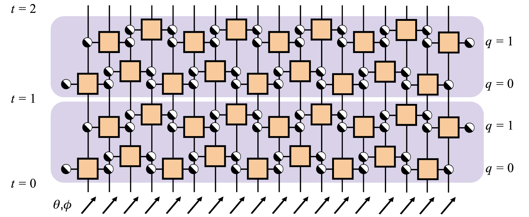
Some time ago, I told you about quantum cellular automata (QCA). These quantum machines are built from one-dimensional strings of qubits. A qubit changes its state depending on the state of its two nearest neighbors. Different rules are encoded into three-qubit gates that change a central qubit based on the state of its left and right neighbors. Some rules induce change for many combinations of neighbor states. Others, less. We apply this neighborhood-constrained update in two waves, first to every other qubit, then to the ones skipped in the first wave. This is a common quantum circuit structure called a brickwork pattern. We call one rule the Goldilocks QCA: A qubit is updated if one of its neighbors is a 0 while the other is a 1 (activity); otherwise the qubit does not change its state (inactivity).
The first figure from our recent paper illustrating the Goldilocks QCA brickwork circuit. Orange boxes represent unitary gates. Half-white-half-black circles represent the Goldilocks neighborhood constraint. Some choices for the unitary gate result in free fermion dynamics. Most choices are consistent with chaos.
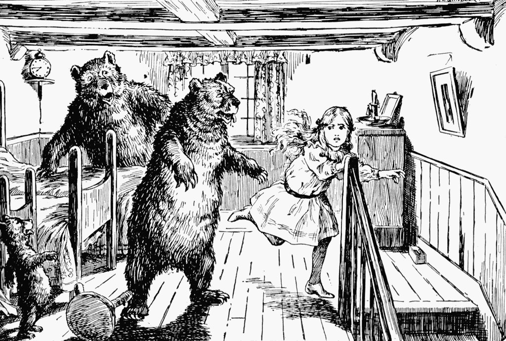
Repeating brickwork layers of the Goldilocks rule, we found, balances activity and inactivity to be “just right,” as Goldilocks might say. Striking this balance produced surprisingly rich patterns of quantum correlation. The same type of network structure is found in complex classical systems like metabolic pathways, social networks, and brain activity. What’s more, the observed patterns of connectivity persist through thousands of circuit layers while other QCA tend towards uniformity.
Goldilocks in a state of activity. Published by The Grolier Society, 1912
Our new paper, Integrability of Goldilocks quantum cellular automata, answers a question that’s been lurking underneath that first result for the last several years. Why does this balance produce such rich and persistent structure? Some Goldilocks QCA, we prove, map onto free fermions, one of the simplest examples of exactly solvable quantum dynamics. How does uncovering this simplification explain the persistent complex patterns? The answer follows from the concept of conservation laws. Piecing together this understanding required assembling an international team of experts who generously shared their knowledge and time. I’ll tell a bit of this scientific story through the lens of our collaboration’s history.
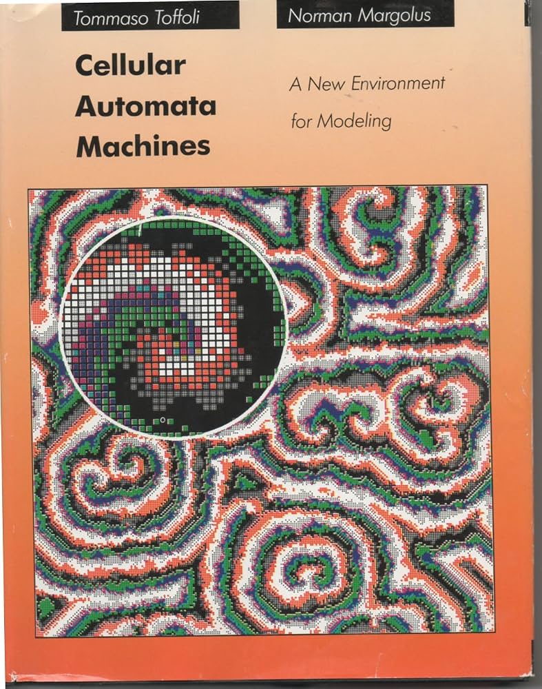
A key inspiration for this work started with a May 2020 video call with Norman Margolus, an MIT-affiliated researcher and pioneer of using cellular automata to model real systems. In the 1980s he worked on a custom computer chip called CAM-6, and later CAM-8, that was dedicated to simulating massive arrays of cellular automata with the limited computational resources of the era2. He proudly showed us beautiful pictures of cellular automata simulating phenomena like optical refraction and chemical reactions.
Cellular automata book by Norman Margolus. His coauthor’s name may also be familiar to those with quantum-circuit experience. Published by MIT Press, 1987.
He told us a story about trying to mimic fluid flow with the simple local rules of classical cellular automata. These models, called lattice gas automata, were first defined on a square lattice. While they did show fluid-like behavior, these models did not quite correctly conserve momentum3. Moving to a hexagonal lattice fixed up these problems and the community was able to devise cellular automata that quantitatively modeled continuum fluid flow.
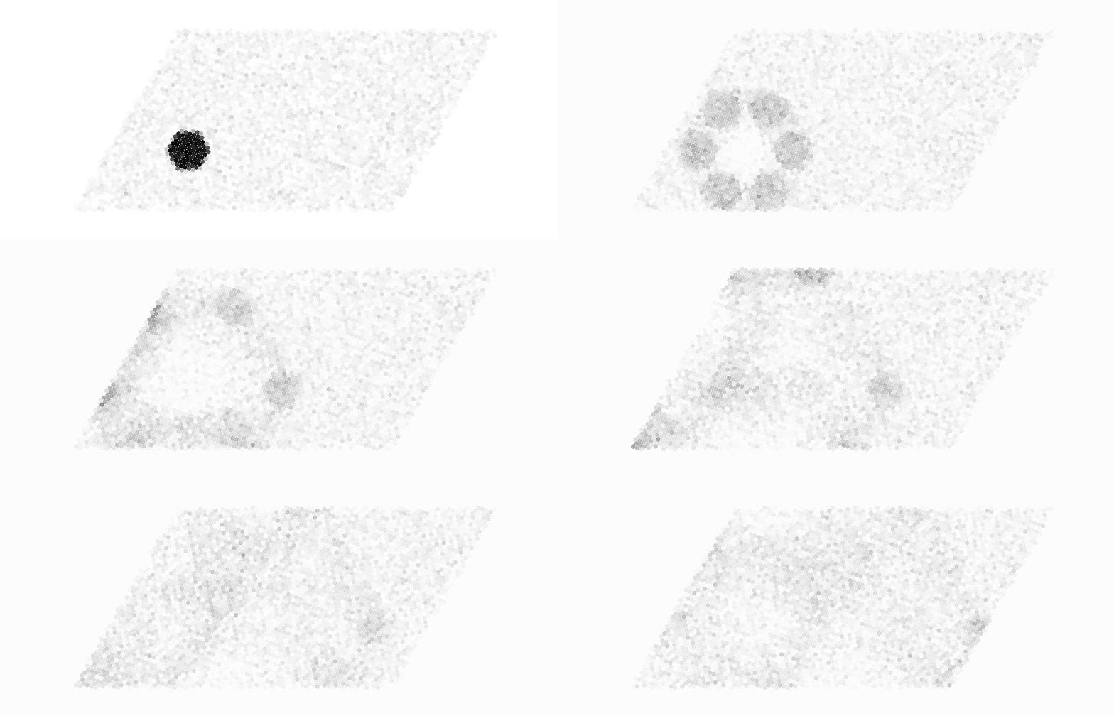
The author’s primitive lattice-gas cellular automaton showing an initial high-density region displaying wave-like propagation, reflection, and diffusion into a low-density background.
Part of that story stuck with me: conservation laws are fundamental ingredients of a physical model. Our Goldilocks quantum cellular automata, we observe, exhibit persistent complex structures. Could some conservation law be behind these observations? If found, could these conservation laws be harnessed for more efficient simulations? Going even further, could there be enough conservation laws to exactly solve the dynamics (at least in principle)? This property would buy the system membership in a special class called integrable systems.
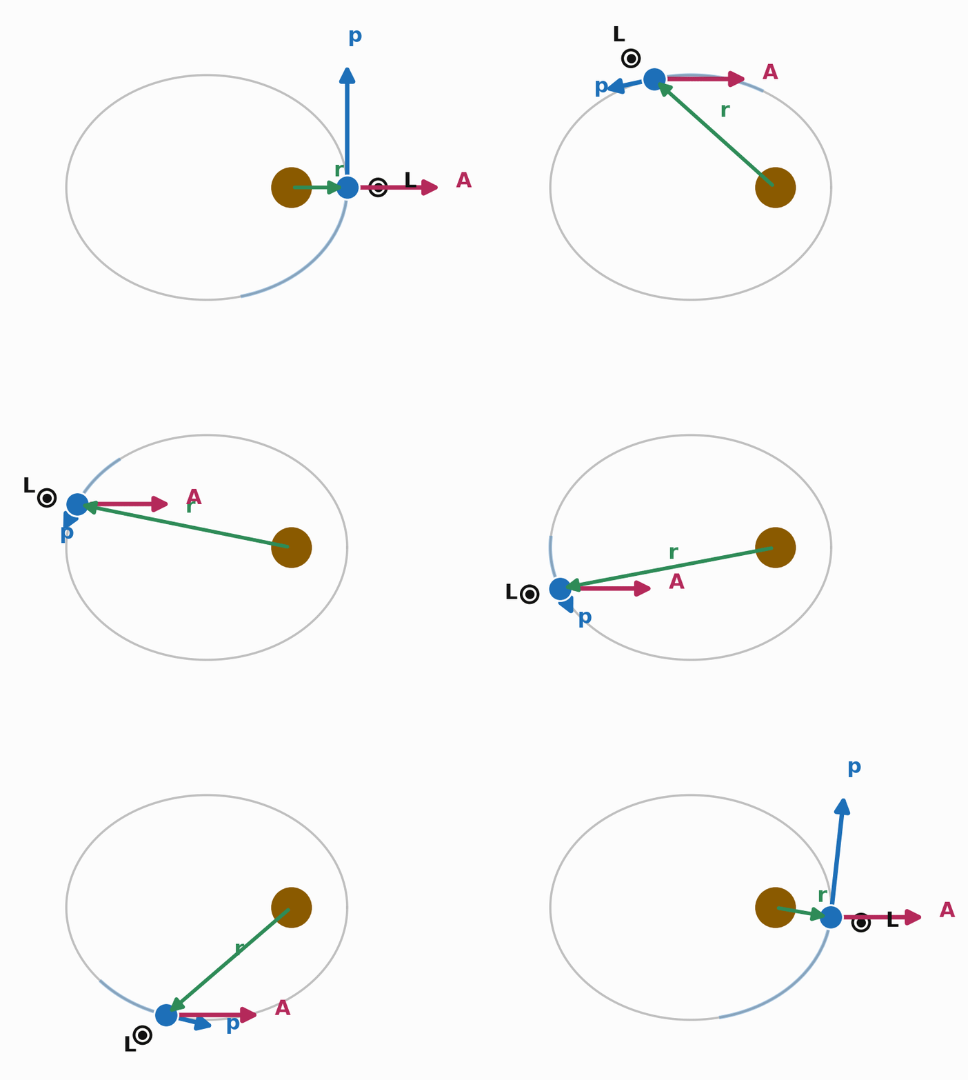
An integrable system conserves enough quantities, often called charges in the quantum setting, that you can compute its future state from its conservation laws and its initial conditions. Two-body gravitational orbits are a classic example. The initial positions and velocities set the orbital energy and angular momentum in the center-of-mass reference frame. Those two conserved quantities let you write down an exact equation for the orbit’s shape.
A familiar integrable system from classical mechanics: the two-body gravitational orbit. Angular momentum L=r x p is conserved. So are the total energy and the Runge-Lenz vector A.
A chaotic system, by contrast, may conserve energy and even a few other quantities, but not enough for us to solve for the state arbitrarily far in the future. To find out what a chaotic system does, you have to evolve the equations of motion approximately—one small time step at a time. Chaotic systems are the norm in nature; integrable ones are rare. To illustrate their qualitative differences, compare the regularity of the above orbit to the trend towards uniformity in the above lattice-gas simulation. In the quantum regime, physicists still don’t fully agree on the precise definition of integrability, though conservation of many independent quantities is a strong indicator.
In August 2020, Nicole emailed Lorenzo Piroli about his preprint on QCA, now published as Phys. Rev. Lett. 125, 190402. Lorenzo was a postdoc at the Max Planck Institute for Quantum Optics in Garching, Germany when we first met. He is now an associate professor at the University of Bologna and expert in many-body quantum dynamics. The correspondence that unfolded set the blueprint for the research effort that followed. One of us would ask a question, and Lorenzo would respond incredibly fast with accurate and useful detail. He started working with us to understand why the Goldilocks QCA dynamics appeared so unique. Lorenzo would suggest computations, I would implement them, and we would discuss what the results meant.
Then came an echo of the collaboration’s inception. In May 2021, Nicole pointed out a relevant preprint from Tomaž Prosen, now published in Chaos 31, 093101. Tomaž is a Slovenian physicist at the University of Ljubljana and a leading researcher in the fields of quantum chaos and integrability. I sent an email about the connections between our work and his. He responded with enthusiasm. He shared some code that would, through exhaustive search, find quantities conserved by our QCA.
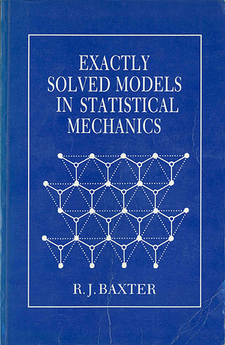
The code’s brute-force approach meant the algorithm could only find conservation laws defined over, at most, a 5-qubit subsystem. A tantalizing signal emerged: the number of conserved quantities supported by 5 qubits exceeded the number supported by 3 qubits. Having more and more conserved quantities as you look at larger neighborhoods is a signature of integrability. Soon after, Tomaž proved one of our Goldilocks QCA is integrable using a well-established toolkit from statistical mechanics called Yang-Baxter integrability. He built a parametric transfer matrix, essentially a machine that spits out a new conserved quantity every time you turn its mathematical crank4.
Rodney Baxter’s classic textbook. Published by Academic Press, 1982
But there was a wrinkle. The transfer matrix generates charges that mutually commute, meaning you can measure them simultaneously. For example, you can know a quantum particle’s kinetic energy and momentum simultaneously because those operators commute. Yet, the search algorithm kept finding charges that did not commute with each other, like a particle’s position and momentum. The only explanation was that our QCA has more charges than the transfer matrix method guarantees, and more than are minimally required for integrability. This extra-conservation-law property, called superintegrability, also shows up in two-body gravitational orbits. In addition to energy and angular momentum, orbits conserve the Runge-Lenz vector. Nicole is an expert on noncommuting charges, so this is where one of her main research efforts entered the QCA collaboration.
Next came a key insight from Lorenzo: the automaton we had been considering was one member of a larger family of integrable Goldilocks QCA. He showed this using a Jordan-Wigner transformation, a mathematical dictionary that translates between the language of qubits and the language of fermions. Complexity in the qubit language transformed into simplicity in the fermion language. Under this translation, our QCA mapped to noninteracting, or free, fermions: particles that never bump into or influence each other. That lack of interaction is what makes free-fermion dynamics easy to calculate. A system of free fermions is a well-known example of superintegrability.
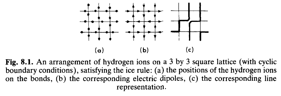
Along the way, Lorenzo recruited his friend and collaborator Eric Vernier, a CNRS researcher based in Paris, France. He is an expert on vertex models. The classical version of the six-vertex model was developed in the 1930s to explain a troubling mystery: Water ice appears to have more entropy than permitted by the third law of thermodynamics at near-zero temperature. In the six-vertex model, a water molecule’s oxygen atom is envisioned at every vertex in a square lattice. Each molecule contributes two hydrogen ions, to use Baxter’s terminology, that fall along the lattice edges. Intermolecular hydrogen bonds between adjacent molecules slightly alter the intramolecular O-H bonds. To maintain electrical neutrality, each oxygen (lattice vertex) has two nearby and two far-away hydrogen ions (four edges), leading to six possible ice vertices. The vertices are commonly visualized in three ways: 1) as the dots representing hydrogen ions located on edges near or far from each vertex, 2) as electric dipole arrows pointing into (“ion is close”) or out of (“ion is far”) each vertex, or 3) as thick (downward- and leftward-pointing dipoles) and thin (upward- and rightward-pointing dipoles) edges. Despite the model’s simplicity (2D square lattice) compared to real ice (3D tetrahedral lattice), it agrees with experimentally measured entropy values to better than 2%.
This figure appears in chapter 8 of R.J. Baxter’s book. It shows three visualizations of the same ice crystal.
More recently, vertex models have been adapted from two-dimensional classical crystals to one-dimensional quantum systems that evolve in time. Eric showed us how the ice vertices relate to QCA circuit rules. In doing so, Eric uncovered an even larger set of integrable Goldilocks QCA than that found by Lorenzo. Eventually, Lorenzo’s Jordan-Wigner transformation method and Eric’s six-vertex method agreed on the complete family of integrable Goldilocks QCA.
Representation of the six ice vertices from our recent paper (rotated 45 degrees from the lattice shown above). The a, b, and c variables represent the classical statistical weight or the quantum transition amplitude for each vertex type.
We finally had our Avengers-style collaboration: individual heroes brought together to wield their unique strengths. With Lincoln’s supervision, I developed the QCA models and performed the computations. Lorenzo found the Jordan-Wigner transformation. Tomaž found the first signals of integrability and delivered a set of conservation laws. Nicole brought her expertise in quantum thermodynamics, clarifying how the noncommuting charges constrain dynamics. Eric made the six-vertex connection. We drafted and redrafted the paper until it balanced the scientific story, the analytical derivations, and the numerical evidence.
Our team collaborated over six years. Art by Barry Windsor-Smith. Published by Titan Comics, 2024
Because the discovered family of Goldilocks QCA maps to free fermions, we can efficiently simulate them classically. I simulated 256 qubits on my laptop this way. These large simulations were satisfying: I had worked with this model for years with an order of magnitude fewer qubits and even saw the dynamics implemented on Google’s Sycamore-era hardware with 23 qubits. Most Goldilocks QCA are consistent with chaos rather than integrability, and therefore hard to simulate classically. Therefore, our work gives experimentalists a tunable model: dial in integrable dynamics for something checkable at large qubit number. Set up chaotic dynamics for a potential demonstration of quantum advantage.
While preparing this post, I opened my old email account to check the timeline set out above. I looked through nearly six years of email chains, some with hundreds of messages, full of logistics for coordinating each author’s ever-changing time zone, and dozens of calculations and results that never made it into the paper. This collaboration helped me grow as a researcher in a big way.
I found old emails where Nicole was coaching me on messaging potential collaborators. I can hardly believe she dedicated so much effort to mentoring me. We have never met in person, despite our shared work starting when I was an undergraduate and she was a graduate student more than a decade ago. If you know Nicole, you can probably believe it easily. I had similar moments with each collaborator. They all gave their time and expertise generously over the many years this paper took to come together.
As I continue my efforts in experimental physics, I will pay forward the effort and generosity shared with me by this collaboration. I may even keep my theoretical-physics license for a while longer.
“By day” doesn’t mean “by daylight.” Laser labs are almost always in a windowless basement. ↩︎
CAM-6 featured 32 kB of cell-state memory (CAM-8 had 8 MB ), far less than the memory currently used by this author’s numerous open browser tabs. ↩︎
The coarse-grained momentum flux tensor was anisotropic. ↩︎
Logarithmic derivatives of the parametric transfer matrix generate the conserved charges. ↩︎
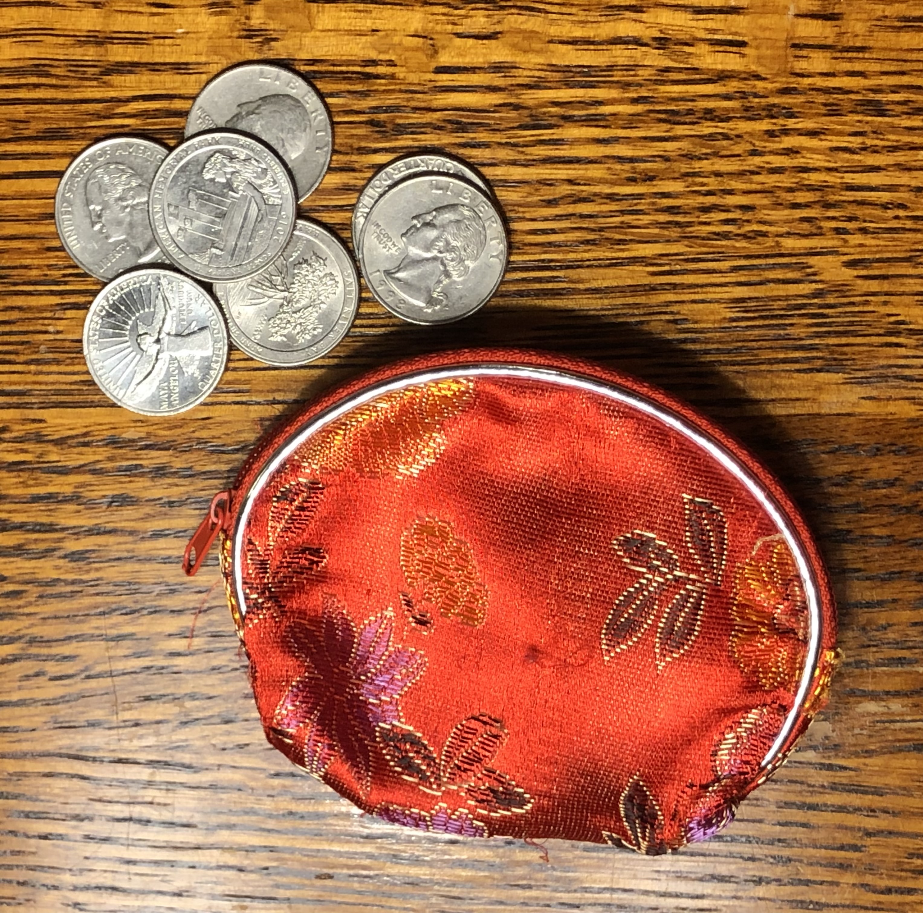
In my closet, in a basket labeled “Random stuff,” sits a bag of quarters. They total only a few dollars, but their worth to me exceeds their monetary value. I received the quarters from Mark Wise.
Mark taught a course about the Standard Model of particle physics at my master’s program at the Perimeter Institute for Theoretical Physics, near Toronto. Perimeter borrowed him from Caltech, to whose faculty he belonged. Mark had grown up in Canada and studied at the University of Toronto; so he didn’t mind visiting Canada even in the depths of winter.
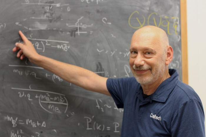
What would Mark have minded? He projected a mild manner—an innocuousness—that suited his sense of humor, which he often directed at himself. Mark had a bald patch and glasses, and he wore a mustache. Physics jokes and science-fiction references decorated his T-shirts, one of which he wore beneath a black suit jacket to our first class. His voice was nasal; it grated a little. But I relished listening to Mark’s lectures.
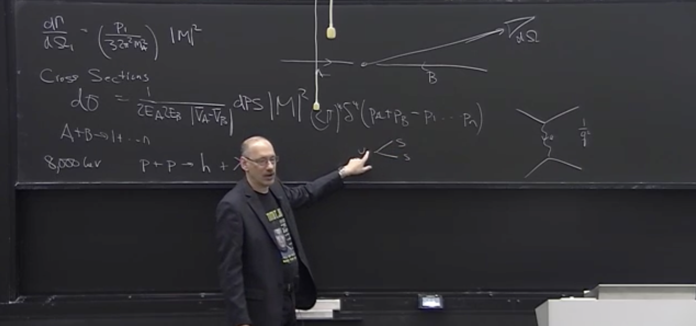
Mark’s lecturing exemplified clarity, because he knew particle physics so deeply. When he walked us through its Lagrangians and scattering diagrams, his conclusions seemed inescapable. His lectures’ logic and structure appealed to me as someone who’s been hyper-organized since at least fourth grade.
Yet Mark cared about us students beyond the requirements of pedagogy. His T-shirts invited conversation from those who arrived to class early. Whenever a student answered or asked a question, he tossed them a quarter. Sometimes, he’d pause to examine the quarter, deliberate about whether to toss a Canadian quarter or an American one, or opine about the motto printed on the coin. (Mark confessed to having lower standards than those ingrained in the New Hampshire state motto, “Live free or die.” Where he came from, “We just wanna live!”)
Some days, Mark found little change in his pocket and announced that he needed to return to the bank for more quarters. The announcements sounded like complaints. He didn’t need to return to the bank, though, as nobody needs to bring doughnuts to the office for sharing.
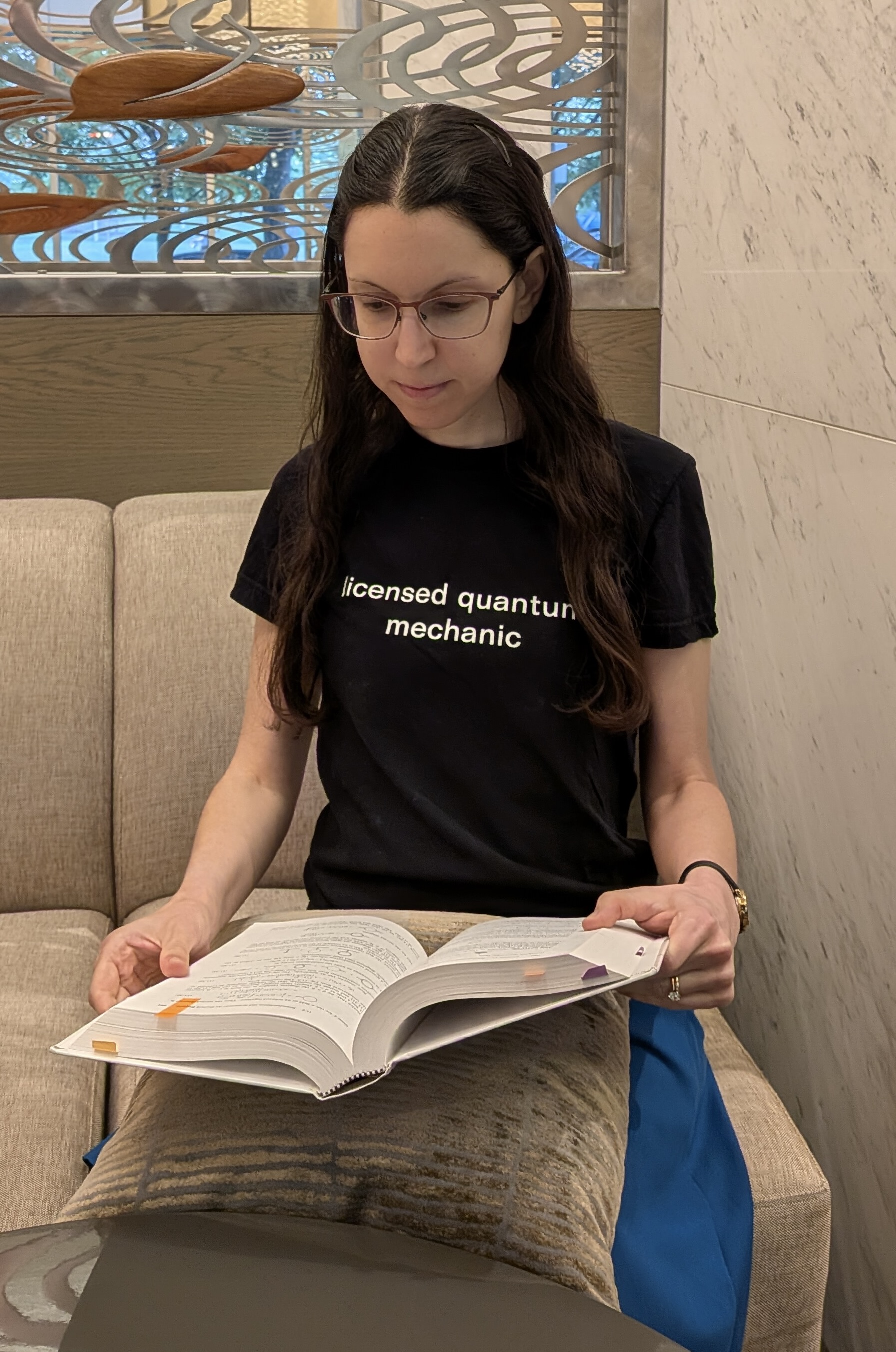
I discovered the icing on the doughnut two years later, as a PhD student at Caltech. I sat in on part of a quantum course taught by Mark. To every student who completed the course, Mark gave a T-shirt that read, “Licensed quantum mechanic.” I received a T-shirt, although I only sat in on part of the course. I’ve never worn it, because I’ve wanted never to wear it out.
In 2024 and 2025, I co-taught a course on quantum-steampunk creative writing. Students learned about quantum physics, quantum technologies, and thermodynamics. Quanta are discrete units. For example, a photon is a quantum of energy. I illustrated quanta with coins, which are discrete units of money. From then on, I tossed a quarter to every student who answered or asked a question about quantum physics. (I joked that I should have tossed pennies, the minimal units of money, but chose quarters because inflation had been high recently.) I adapted Mark’s tradition to thermodynamics—the study of energy—by tossing Hershey’s kisses—dense packets of energy.
Before moving out of Caltech, I said goodbye to Mark. He worked among the high-energy theorists, rather than the quantum information or condensed-matter theorists, so I had to hunt down his office. He smiled and made a joke, of course.
Mark passed away this summer. His Caltech colleague John Preskill published a eulogy as a blog post here. (I learned from John’s post that inflation led Mark to upgrade his quarters to dollar coins. So much for feeling generous about upgrading from pennies to quarters.) When asked about the student experience at Caltech, Mark would say, “Caltech is heaven for professors.” Irony would creep into his voice and body language as he’d continue, “Doesn’t that mean it’s heaven for students, too?” I worked my rear off as a student at Caltech and Perimeter, but I’d call both environments fairly heavenly. Mark and his ilk are reasons why.
Mark Wise, the John A. McCone Professor of High Energy Physics at Caltech, passed away on July 10 at age 72. At a recent memorial service, John Preskill made these remarks.
I’m John Preskill, Mark’s colleague on the Caltech physics faculty for more than four decades. Our friendship goes back even farther. My wife Roberta and I met Mark and Jackie not long after they arrived at Harvard in 1980. We’ve been friends since then. We attended the bris for both Barry and Jonathan during those Harvard days. Mark and Jackie have two boys and we have two girls who are a few years younger, who were thrilled to connect with Barry and Jonathan when the families would get together for occasions like Passover or Hanukkah or Thanksgiving. When the kids were little, Mark and I would sometimes muse about the potential for forging even closer family ties if those relationships blossomed.
That didn’t happen. But Mark would preside at each Seder with a light hand, sprinkling the occasion with corny jokes as was his style, and Jackie would be determined to make it to the end of that customized family-friendly Haggadah she had meticulously prepared. The children, meanwhile, would be wondering when they’d be able to continue their game of sock baseball.
Many of you know that Mark was deeply dedicated to his family and friends. I’ll make some brief remarks about three facets of Mark I know especially well: Mark the scientist, Mark the teacher and mentor, and Mark the colleague and friend.
Because of his self-deprecating manner, those of you who are not scientists may not appreciate Mark’s stature as a physicist. He was one of the most influential figures in theoretical particle physics of his generation. It was not obvious things would turn out that way. Growing up in Toronto, Mark was an indifferent student, and his poor grades reflected that lack of interest. As a 9th grader, though, it struck him that he better change his ways and figure out how to make something of his life. He liked sports — the possibility of being a professional athlete was briefly considered, but discarded. Somehow he decided that science would be a better fit. I’m not sure why — he had recently failed math. But he worked hard and had inspiring teachers, so by the time he finished high school Mark was an excellent student, and he sailed into the University of Toronto well prepared to major in physics,
At U of T, Mark came under the influence of a young professor, Nathan Isgur, who would later become his close research collaborator. Under Nathan’s guidance, Mark sought admission to the PhD programs of the most prestigious US research universities, intent on a career devoted to deep exploration of the fundamental laws of physics. He was rejected everywhere he applied. He should have been discouraged. But he wasn’t. Mark shrugged and said: “It’s okay. I’ll stay another year in Toronto, I’ll get a master’s degree, I’ll apply again and I’ll get in somewhere.” And that’s what happened. He went to Stanford, where, under the kind tutelage of Fred Gilman, Mark took off like a rocket. Hired to the Caltech faculty in 1982, he was a tenured full professor three years later at the age of 31, and appointed as the John A. McCone Professor of High Energy Physics while still in his 30s.
Mark liked action movies, such as those starring Arnold Schwarzenegger or Clint Eastwood. In serious moments, we would sometimes ponder together why we’re successful at what we do, and Mark would always quote Clint Eastwood as Harry Callahan in Magnum Force: “A man’s got to know his limitations.” We would both laugh, but those were words of wisdom. Mark understood what he did well as a research scientist and what he was less good at. Finding problems he could solve that would have interesting consequences for experiments that had been done or could be done was where he excelled – he did it again and again. Mark never lost his zest for calculating things, often by hand with pen and paper, his head resting on one arm with his glasses pushed up onto his forehead as he scribbled. Getting to an answer that was experimentally relevant never stopped giving him a thrill.
Mark also never lost his sense of appreciation for the teachers and mentors who had inspired and helped him. Perhaps that’s why he became such a dedicated teacher and mentor himself. It’s hard to impress Caltech students, but Mark’s lectures where extremely popular, not just for their pedagogical value but also for the humanity and humor he displayed. Students had to pay attention because otherwise one might miss the jokes, which inevitably became known as “Wisecracks.” There is even an account on X with the handle @MarkWiseSays, curated by students who want to preserve Mark’s pithy lessons in physics and in life.
For example, Mark might say: “If you really get depressed, I recommend diagonalizing a 2×2 matrix.” For physics students, this is both funny and sage advice. Or he might say. “This calculation will knock your socks off.” A cliché you might hear from anyone. But who besides Mark would then proceed to remove his shoes, rip off his socks, hurl them at the blackboard, put his shoes back on and resume lecturing?
Most famously, Mark would come to class with an ample supply of coins. He would ask the class questions, sometimes about physics and sometimes random trivia, rewarding a student who gave an answer Mark approved of by tossing a coin. At first the coins were quarters. But Mark, who had a scholarly interest in finance as well as physics, eventually felt that due to inflation he needed to upgrade to dollar coins. These are harder to come by, so it took frequent visits to the bank to make sure he wouldn’t run out. His antics in class made Mark human and approachable, and students responded. Mark felt that many Caltech students don’t fully realize how smart they are. He saw part of his job as building their self-confidence and relieving their stress.
As a colleague and mentor to graduate students and postdoctoral scholars, Mark was highly collaborative. He believed that interactions with others sparked his creativity. He was never at all pompous. I know this started early. When we were in the Harvard Society of Fellows we were obligated to have dinner with the Senior Fellows on Monday nights. It was a rather stuffy occasion. And, though I don’t think they do this anymore, after a sumptuous meal we would literally retire for brandy and cigars. Once, while puffing on his cigar after dinner, Mark had an inspiration. He gathered up a few junior fellows and led them to a theater for a movie he thought everyone should see right away. The movie was Conan the Barbarian. And everyone had a blast. That was a perfect Mark moment.
As the news about Mark has spread, accolades have poured in from physicists all over the world. He was admired not just for his scientific brilliance, but almost as much for his quirky sense of humor and his kindness. Mark was a wonderful friend to many of us. When you were with him, you were sure to laugh and feel good. He touched the lives of countless colleagues, students and friends. We miss him terribly but there are so many memories that we’ll cherish. We are all so very fortunate to have known and loved Professor Mark Wise.
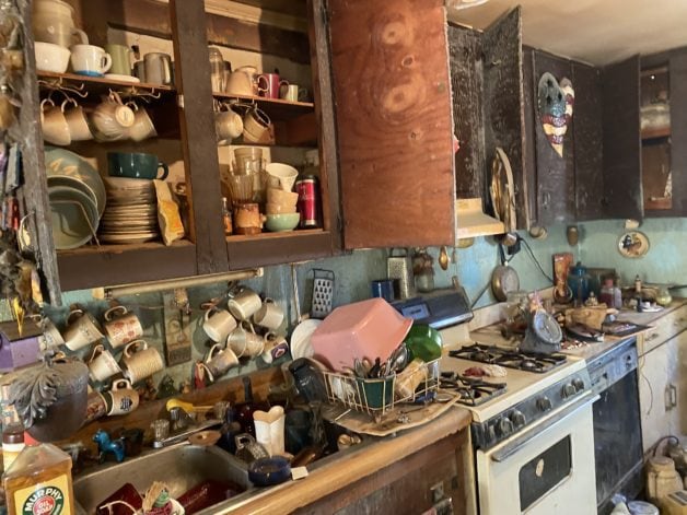
When I was pursuing a PhD at Caltech, so was my friend Jeremy. He used to throw a dinner party every few months. The email invitations welcomed friends to partake of his cooking and, if we wished, to help him cook. I didn’t help cook; but, when I arrived, the mess of pots and pans drew me to the kitchen like vinegar drawing a pathological fly. I couldn’t sit still while cookware needed cleaning, so I scrubbed and rinsed the pans and spoons and bowls. Jeremy, an applied-physics student, commented on my adeptness at decreasing entropy.
It’s the story of my life, I replied.
In fourth grade, my classmates and I cleaned our desks every Friday afternoon. Once a student finished, my teacher dismissed him or her onto the playground. My neighbor’s desk horrified me like the disaster in a hurricane’s wake, so I neatened his desk after finishing with mine.1 Another friend requested the same favor. A third classmate offered to pay me for cleaning his desk, but I’d have undertaken the chore for its own sake. Ordering the world offered me fulfillment.
From cleaning a fourth-grade desk, I progressed to pursuing a PhD in theoretical physics. The two pursuits might seem to resemble each other no more than Dr. Jekyll and Mr. Hyde; yet, to me, the path between them is but a step. I trained as a theoretical physicist because I love organizing ideas. Caltech paid me to build models, propose definitions and theorems, and structure proofs—to dream up ideas and identify the optimal arrangements for them. I needed that pay, being an adult, as I hadn’t needed my fourth-grade classmate’s desk-cleaning fee. Yet I organized ideas for the same reason that drove me to organize my neighbor’s notebooks.
Many people have called entropy a measure of disorder. To see why, imagine that Jeremy’s crew has used thirty utensils while cooking. The chefs can have scattered the utensils across the kitchen in many ways: they may have dropped forks on the floor, left spoons in the sink, arranged spatulas on the drying rack, or filled a vase with knives like a modern-art bouquet. In few of these configurations do the forks lie in their compartment of the utensil drawer, the spoons lie in their compartment, etc. We call such configurations neat. Most of the other configurations, we call messy.
A system’s entropy is the number of configurations consistent with known large-scale properties of the system, such as the number of forks.2 More configurations are consistent with messiness (and a fixed number of forks and so on) than with neatness (and the same number of forks and so on). Messiness tends to correlate with high entropy. People often say, therefore, that entropy quantifies messiness. Hence Jeremy’s complimenting me on my decreasing of entropy.
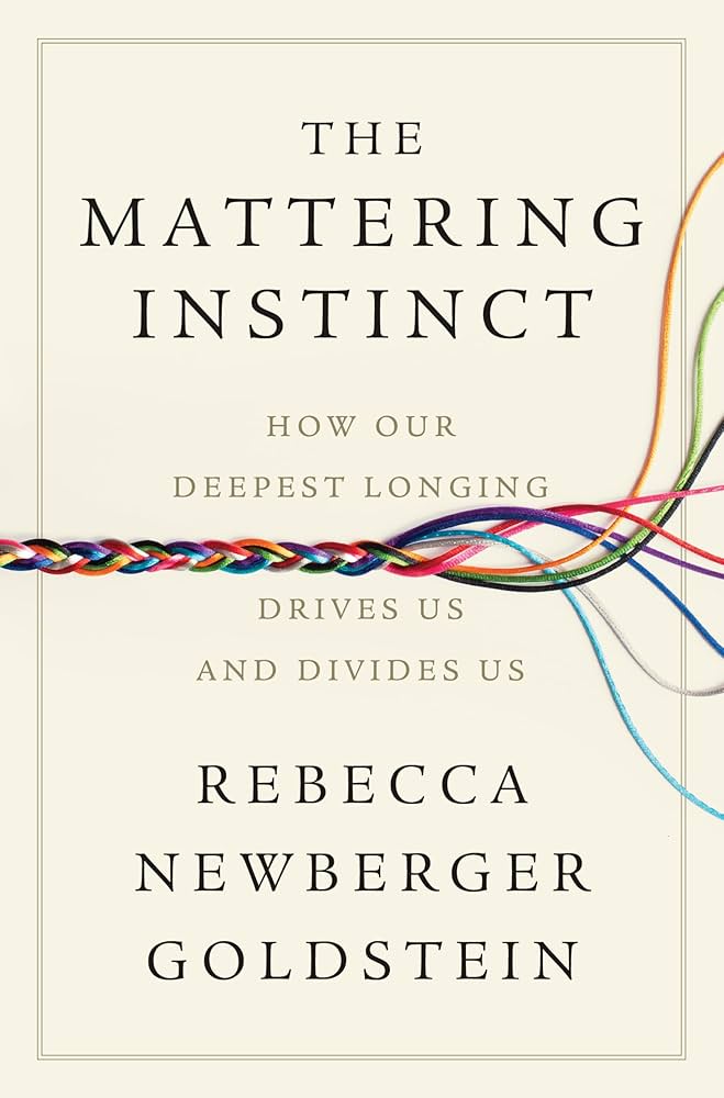
Jeremy’s dinner parties came to mind as I read the book The Mattering Instinct, published by Rebecca Newberger Goldstein this January. Rebecca is a philosopher of science and a writer. I had the good fortune to meet her through my undergraduate mentor Marcelo Gleiser, who’s had another cameo or two on Quantum Frontiers. Rebecca’s latest book covers what she calls the mattering instinct: the longing to know that we matter.
We spend scads of energy and time on securing our “survival and flourishing,” as Rebecca says. We feed ourselves; work to earn money to purchase food; clean, shelter, and clothe ourselves; ingrain ourselves in societies that offer some degree of security; and more. Do we deserve all this effort? We long for assurance that, in the immortal words of L’Oreal, we’re worth it.
Survival and flourishing, Rebecca writes, requires us to decrease entropy. Every closed, isolated system’s entropy increases or remains constant, according to the second law of thermodynamics. Entropy increases as a system becomes more uniform, loosely speaking. The system’s particles spread out across space, these particles’ temperature comes to equal those particles’ temperature, and so on. In contrast, your body exists because its particles clump together in a certain shape consistently. You withstand heat waves and snow because homeostasis maintains your temperature despite your environment’s temperature. You keep your body’s entropy low to survive. Rebecca therefore casts us as fighting entropy.
As a thermodynamicist, I agree with Rebecca. Yet I also adore entropy. It helps explain why time flows, quantifies uncertainty, and determines the maximal efficiencies with which we can perform tasks such as communication. What versatility and richness! Entropy also embodies tension and subtlety: its mathematical definition looks obscure at first glance, yet entropy helps explain familiar phenomena such as aging. For these reasons, before beginning my PhD, I told a potential advisor that I could imagine devoting the next five years of my life to entropy.
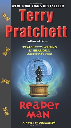
I therefore aspire to rehabilitate entropy’s reputation. Novelist Terry Pratchett endeared mortality to millions of readers through anthropomorphism. His character Death, a mainstay of the Discworld series of novels, elicits empathy and fondness. I won’t anthropomorphize entropy here,3 but I aim to replace conflict with cooperation in the narrative above. To survive and flourish, I hold, we partner with entropy. How? We create oodles of entropy in our environments. This entropy increase offsets the entropy decrease that supports life.
For example, imagine working at a desalination plant. You’d process high-entropy water throughout which salt has spread. You’d concentrate the salt in a tiny region, reducing the water’s entropy. This reduction, producing fresh water, could support your city’s drinking, cooking, and toothbrushing needs.
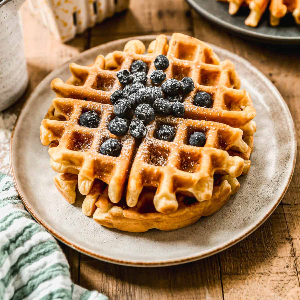
To reduce the water’s entropy, you’d create loads more entropy. You’d eat breakfast before work, consuming energy stored neatly in your waffle’s chemical bonds. Your body would later break the bonds, releasing the energy. Some energy would power your muscles, so you could program the desalination system, test its output, etc. But much of the chemical energy would transform into heat radiated by your body. The heat would warm up the air molecules around you, magnifying their random jigglings and jostlings. You’d increase the entropy of the air—your environment—to decrease the water’s entropy. The air’s entropy increase would outweigh the water’s entropy decrease.
Organisms survive and flourish by producing entropy in their environments. In fact, organisms have a knack for generating entropy. Entropy and life thereby further each other. A glass-half-full thinker could conclude that we partner with entropy.
So did I partner with entropy as a PhD student, applying it to solve problems in quantum information theory and thermodynamics. So did I partner with entropy in fourth grade and at Jeremy’s apartment, deriving satisfaction from my cleaning. Rebecca would call these activities’ ultimate aim (beyond the aim of, e.g., not sitting beside a pigsty in fourth grade) mattering. She writes that we reduce entropy (within our immediate vicinities) to satisfy the mattering instinct. Rebecca’s proposition describes my behaviors with uncanny precision, I realized upon reading her book.
Which I’ve now finished. So pardon me while I return to washing forks in the quantum kitchen of the universe.
With thanks to Jeremy for his friendship…and food.
1I also ensured that my neighbor brought home, every afternoon, the sweater he’d brought to school that morning. Before I took charge, he’d ended up with three forgotten sweaters crammed into his cubby.
We are now at an exciting point in our process of developing quantum computers and understanding their computational power: It has been demonstrated that quantum computers can outperform classical ones (if you buy my argument from Parts 1 and 2 of this mini series). And it has been demonstrated that quantum fault-tolerance is possible for at least a few logical qubits. Together, these form the elementary building blocks of useful quantum computing.
And yet: the devices we have seen so far are still nowhere near being useful for any advantageous application in, say, condensed-matter physics or quantum chemistry, which is where the promise of quantum computers lies.
So what is next in quantum advantage?
This is what this third and last part of my mini-series on the question “Has quantum advantage been achieved?” is about.
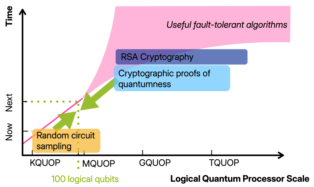
The 100 logical qubits regime I want to have in mind the regime in which we have 100 well-functioning logical qubits, so 100 qubits on which we can run maybe 100 000 gates.
Building devices operating in this regime will require thousand(s) of physical qubits and is therefore well beyond the proof-of-principle quantum advantage and fault-tolerance experiments that have been done. At the same time, it is (so far) still one or more orders of magnitude away from any of the first applications such as simulating, say, the Fermi-Hubbard model or breaking cryptography. In other words, it is a qualitatively different regime from the early fault-tolerant computations we can do now. And yet, there is not a clear picture for what we can and should do with such devices.
The next milestone: classically verifiable quantum advantage
In this post, I want to argue that a key milestone we should aim for in the 100 logical qubit regime is classically verifiable quantum advantage. Achieving this will not only require the jump in quantum device capabilities but also finding advantage schemes that allow for classical verification using these limited resources.
Why is it an interesting and feasible goal and what is it anyway?
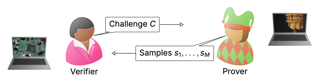
To my mind, the biggest weakness of the RCS experiments is the way they are verified. I discussed this extensively in the last posts—verification uses XEB which can be classically spoofed, and only actually measured in the simulatable regime. Really, in a quantum advantage experiment I would want there to be an efficient procedure that will without any reasonable doubt convince us that a computation must have been performed by a quantum computer when we run it. In what I think of as classically verifiable quantum advantage, a (classical) verifier would come up with challenge circuits which they would then send to a quantum server. These would be designed in such a way that once the server returns classical samples from those circuits, the verifier can convince herself that the server must have run a quantum computation.
The theoretical computer scientist’s cartoon of verifying a quantum computer.
This is the jump from a physics-type experiment (the sense in which advantage has been achieved) to a secure protocol that can be used in settings where I do not want to trust the server and the data it provides me with. Such security may also allow a first application of quantum computers: to generate random numbers whose genuine randomness can be certified—a task that is impossible classically.
Here is the problem: On the one hand, we do know of schemes that allow us to classically verify that a computer is quantum and generate random numbers, so called cryptographic proofs of quantumness (PoQ). A proof of quantumness is a highly reliable scheme in that its security relies on well-established cryptography. Their big drawback is that they require a large number of qubits and operations, comparable to the resources required for factoring. On the other hand, the computations we can run in the advantage regime—basically, random circuits—are very resource-efficient but not verifiable.
The 100-logical-qubit regime lies right in the middle, and it seems more than plausible that classically verifiable advantage is possible in this regime. The theory challenge ahead of us is to find it: a quantum advantage scheme that is very resource-efficient like RCS and also classically verifiable like proofs of quantumness.
To achieve verifiable advantage in the 100-logical-qubit regime we need to close the gap between random circuit sampling and proofs of quantumness.
With this in mind, let me spell out some concrete goals that we can achieve using 100 logical qubits on the road to classically verifiable quantum advantage.
1. Demonstrate fault-tolerant quantum advantage
Before we talk about verifiable advantage, the first experiment I would like to see is one that combines the two big achievements of the past years, and shows that quantum advantage and fault-tolerance can be achieved simultaneously. Such an experiment would be similar in type to the RCS experiments, but run on encoded qubits with gate sets that match that encoding. During the computation, noise would be suppressed by correcting for errors using the code. In doing so, we could reach the near-perfect regime of RCS as opposed to the finite-fidelity regime that current RCS experiments operate in (as I discussed in detail in Part 2).
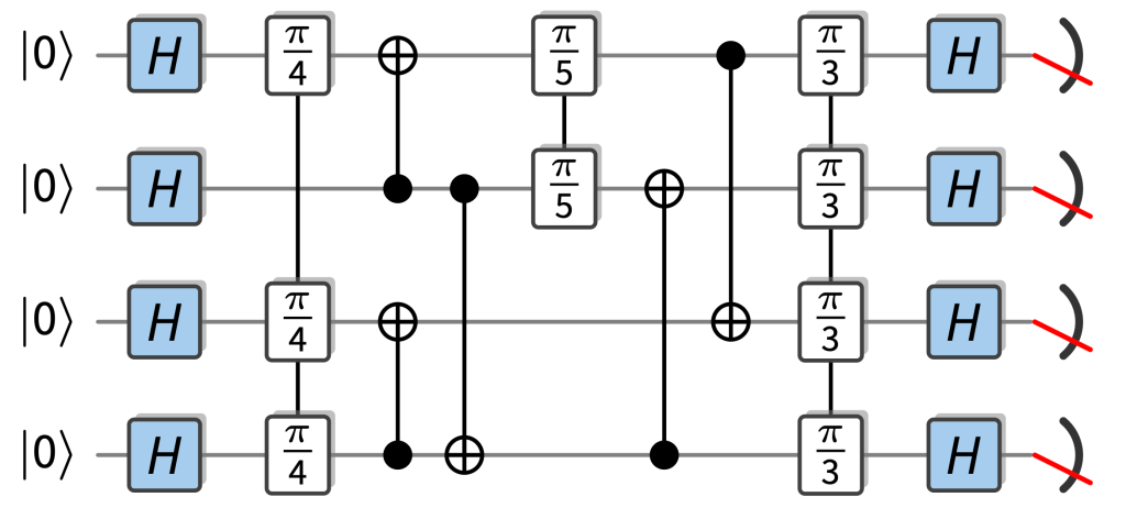
Random circuits with a quantum advantage that are particularly easy to implement fault-tolerantly are so-called IQP circuits. In those circuits, the gates are controlled-NOT gates and diagonal gates, so rotations , which just add a phase to a basis state as . The only “quantumness” comes from the fact that each input qubit is in the superposition state , and that all qubits are measured in the basis. This is an example of an example of an IQP circuit:
An IQP circuit starts from the all- state by applying a Hadamard transform, followed by IQP gates (in this case , some CNOT gates, , some CNOT gates, ) and ends in a measurement in the Hadamard basis.
As it so happens, IQP circuits are already really well understood since one of the first proposals for quantum advantage was based on IQP circuits (VerIQP1), and for a lot of the results in random circuits, we have precursors for IQP circuits, in particular, their ideal and noisy complexity (SimIQP). This is because their near-classical structure makes them relatively easy to study. Most importantly, their outcome probabilities are simple (but exponentially large) sums over phases that can just be read off from which gates are applied in the circuit and we can use well-established classical techniques like Boolean analysis and coding theory to understand those.
IQP gates are natural for fault-tolerance because there are codes in which all the operations involved can be implemented transversally. This means that they only require parallel physical single- or two-qubit gates to implement a logical gate rather than complicated fault-tolerant protocols which are required for universal circuits. This is in stark contrast to universal circuit which require resource-intensive fault-tolerant protocols. Running computations with IQP circuits would also be a step towards running real computations in that they can involve structured components such as cascades of CNOT gates and the like. These show up all over fault-tolerant constructions of algorithmic primitives such as arithmetic or phase estimation circuits.
Our concrete proposal for an IQP-based fault-tolerant quantum advantage experiment in reconfigurable-atom arrays is based on interleaving diagonal gates and CNOT gates to achieve super-fast scrambling (ftIQP1). A medium-size version of this protocol was implemented by the Harvard group (LogicalExp) but with only a bit more effort, it could be performed in the advantage regime.
In those proposals, verification will still suffer from the same problems of standard RCS experiments, so what’s up next is to fix that!
2. Closing the verification loophole
I said that a key milestone for the 100-logical-qubit regime is to find schemes that lie in between RCS and proofs of quantumness in terms of their resource requirements but at the same time allow for more efficient and more convincing verification than RCS. Naturally, there are two ways to approach this space—we can make quantum advantage schemes more verifiable, and we can make proofs of quantumness more resource-efficient.
First, let’s focus on the former approach and set a more moderate goal than full-on classical verification of data from an untrusted server. Are there variants of RCS that allow us to efficiently verify that finite-fidelity RCS has been achieved if we trust the experimenter and the data they hand us?
2.1 Efficient quantum verification using random circuits with symmetries
Indeed, there are! I like to think of the schemes that achieve this as random circuits with symmetries. A symmetry is an operator such that the outcome state of the computation (or some intermediate state) is invariant under the symmetry, so . The idea is then to find circuits that exhibit a quantum advantage and at the same time have symmetries that can be easily measured, say, using only single-qubit measurements or a single gate layer. Then, we can use these measurements to check whether or not the pre-measurement state respects the symmetries. This is a test for whether the quantum computer prepared the correct state, because errors or deviations from the true state would violate the symmetry (unless they were adversarially engineered).
In random circuits with symmetries, we can thus use small, well-characterized measurements whose outcomes we trust to probe whether a large quantum circuit has been run correctly. This is possible in a scenario I call the trusted experimenter scenario.
The trusted experimenter scenario In this scenario, we receive data from an actual experiment in which we trust that certain measurements were actually and correctly performed.
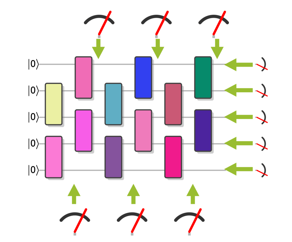
I think of random circuits with symmetries as introducing measurements in the circuit that check for errors.
Here are some examples of random circuits with symmetries, which allow for efficient verification of quantum advantage in the trusted experimenter scenario.
Graph states. My first example are locally rotated graph states (GStates). These are states that are prepared by CZ gates acting according to the edges of a graph on an initial all- state, and a layer of single-qubit -rotations is performed before a measurement in the basis. (Yes, this is also an IQP circuit.) The symmetries of this circuit are locally rotated Pauli operators, and can therefore be measured using only single-qubit rotations and measurements. What is more, these symmetries fully determine the graph state. Determining the fidelity then just amounts to averaging the expectation values of the symmetries, which is so efficient you can even do it in your head. In this example, we need measuring the outcome state to obtain hard-to-reproduce samples and measuring the symmetries are done in two different (single-qubit) bases.
With 100 logical qubits, samples from classically intractable graph states on several 100 qubits could be easily generated.
Bell sampling. The drawback of this approach is that we need to make two different measurements for verification and sampling. But it would be much more neat if we could just verify the correctness of a set of classically hard samples by only using those samples. For an example where this is possible, consider two copies of the output state of a random circuit, so . This state is invariant under a swap of the two copies, and in fact the expectation value of the SWAP operator in a noisy state preparation of determines the purity of the state, so . It turns out that measuring all pairs of qubits in the state in the pairwise basis of the four Bell states , where is one of the four Pauli matrices , this is hard to simulate classically (BellSamp). You may also observe that the SWAP operator is diagonal in the Bell basis, so its expectation value can be extracted from the Bell-basis measurements—our hard to simulate samples. To do this, we just average sign assignments to the samples according to their parity.
If the circuit is random, then under the same assumptions as those used in XEB for random circuits, the purity is a good estimator of the fidelity, so . So here is an example, where efficient verification is possible directly from hard-to-simulate classical samples under the same assumptions as those used to argue that XEB equals fidelity.
With 100 logical qubits, we can achieve quantum advantage which is at least as hard as the current RCS experiments that can also be efficiently (physics-)verified from the classical data.
Fault-tolerant circuits. Finally, suppose that we run a fault-tolerant quantum advantage experiment. Then, there is a natural set of symmetries of the state at any point in the circuit, namely, the stabilizers of the code we use. In a fault-tolerant experiment we repeatedly measure those stabilizers mid-circuit, so why not use that data to assess the quality of the logical state? Indeed, it turns out that the logical fidelity can be estimated efficiently from stabilizer expectation values even in situations in which the logical circuit has a quantum advantage (SyndFid).
With 100 logical qubits, we could therefore just run fault-tolerant IQP circuits in the advantage regime (ftIQP1) and the syndrome data would allow us to estimate the logical fidelity.
In all of these examples of random circuits with symmetries, coming up with classical samples that pass the verification tests is very easy, so the trusted-experimenter scenario is crucial for this to work. (Note, however, that it may be possible to add tests to Bell sampling that make spoofing difficult.) At the same time, these proposals are very resource-efficient in that they only increase the cost of a pure random-circuit experiment by a relatively small amount. What is more, the required circuits have more structure than random circuits in that they typically require gates that are natural in fault-tolerant implementations of quantum algorithms.
Performing random circuit sampling with symmetries is therefore a natural next step en-route to both classically verifiable advantage that closes the no-efficient verification loophole, and towards implementing actual algorithms.
What if we do not want to afford that level of trust in the person who runs the quantum circuit, however?
2.2 Classical verification using random circuits with planted secrets
If we do not trust the experimenter, we are in the untrusted quantum server scenario.
The untrusted quantum server scenario In this scenario, we delegate a quantum computation to an untrusted (presumably remote) quantum server—think of using a Google or Amazon cloud server to run your computation. We can communicate with this server using classical information.
In the untrusted server scenario, we can hope to use ideas from proofs of quantumness such as the use of classical cryptography to design families of quantum circuits in which some secret structure is planted. This secret structure should give the verifier a way to check whether a set of samples passes a certain verification test. At the same time it should not be detectable, or at least not be identifiable from the circuit description alone.
The simplest example of such secret structure could be a large peak in an otherwise flat output distribution of a random-looking quantum circuit. To do this, the verifier would pick a (random) string and design a circuit such that the probability of seeing in samples, is large. If the peak is hidden well, finding it just from the circuit description would require searching through all of the outcome bit strings and even just determining one of the outcome probabilities is exponentially difficult. A classical spoofer trying to fake the samples from a quantum computer would then be caught immediately: the list of samples they hand the verifier will not even contain unless they are unbelievably lucky, since there are exponentially many possible choices of .
Unfortunately, planting such secrets seems to be very difficult using universal circuits, since the output distributions are so unstructured. This is why we have not yet found good candidates of circuits with peaks, but some tries have been made (Peaks,ECPeaks,HPeaks)
We do have a promising candidate, though—IQP circuits! The fact that the output distributions of IQP circuits are quite simple could very well help us design sampling schemes with hidden secrets. Indeed, the idea of hiding peaks has been pioneered by Shepherd and Bremner (VerIQP1) who found a way to design classically hard IQP circuits with a large hidden Fourier coefficient. The presence of this large Fourier coefficient can easily be checked from a few classical samples, and random IQP circuits do not have any large Fourier coefficients. Unfortunately, for that construction and a variation thereof (VerIQP2), it turned out that the large coefficient can be detected quite easily from the circuit description (ClassIQP1,ClassIQP2).
To this day, it remains an exciting open question whether secrets can be planted in (maybe IQP) circuit families in a way that allows for efficient classical verification. Even finding a scheme with some large gap between verification and simulation times would be exciting, because it would for the first time allow us to verify a quantum computing experiment in the advantage regime using only classical computation.
Towards applications: certifiable random number generation
Beyond verified quantum advantage, sampling schemes with hidden secrets may be usable to generate classically certifiable random numbers: You sample from the output distribution of a random circuit with a planted secret, and verify that the samples come from the correct distribution using the secret. If the distribution has sufficiently high entropy, truly random numbers can be extracted from them. The same can be done for RCS, except that some acrobatics are needed to get around the problem that verification is just as costly as simulation (CertRand, CertRandExp). Again, a large gap between verification and simulation times would probably permit such certified random number generation.
The goal here is firstly a theoretical one: Come up with a planted-secret RCS scheme that has a large verification-simulation gap. But then, of course, it is an experimental one: actually perform such an experiment to classically verify quantum advantage.
Should an IQP-based scheme of circuits with secrets exist, 100 logical qubits is the regime where it should give a relevant advantage.
Three milestones
Altogether, I proposed three milestones for the 100 logical qubit regime.
Perform fault-tolerant quantum advantage using random IQP circuits. This will allow an improvement of the fidelity towards performing near-perfect RCS and thus closes the scalability worries of noisy quantum advantage I discussed in my last post.
Perform RCS with symmetries. This will allow for efficient verification of quantum advantage in the trusted experimenter scenario and thus make a first step toward closing the verification loophole.
Find and perform RCS schemes with planted secrets. This will allow us to verify quantum advantage in the remote untrusted server scenario and presumably give a first useful application of quantum computers to generate classically certified random numbers.
All of these experiments are natural steps towards performing actually useful quantum algorithms in that they use more structured circuits than just random universal circuits and can be used to benchmark the performance of the quantum devices in an advantage regime. Moreover, all of them close some loophole of the previous quantum advantage demonstrations, just like follow-up experiments to the first Bell tests have closed the loopholes one by one.
I argued that IQP circuits will play an important role in achieving those milestones since they are a natural circuit family in fault-tolerant constructions and promising candidates for random circuit constructions with planted secrets. Developing a better understanding of the properties of the output distributions of IQP circuits will help us achieve the theory challenges ahead.
Experimentally, the 100 logical qubit regime is exactly the regime to shoot for with those circuits since while IQP circuits are somewhat easier to simulate than universal random circuits, 100 qubits is well in the classically intractable regime.
What I did not talk about
Let me close this mini-series by touching on a few things that I would have liked to discuss more.
First, there is the OTOC experiment by the Google team (OTOC) which has spawned quite a debate. This experiment claims to achieve quantum advantage for an arguably more natural task than sampling, namely, computing expectation values. Computing expectation values is at the heart of quantum-chemistry and condensed-matter applications of quantum computers. And it has the nice property that it is what the Google team called “quantum-verifiable” (and what I would call “hopefully-in-the-future-verifiable”) in the following sense: Suppose we perform an experiment to measure a classically hard expectation value on a noisy device now, and suppose this expectation value actually carries some signal, so it is significantly far away from zero. Once we have a trustworthy quantum computer in the future, we will be able to check that the outcome of this experiment was correct and hence quantum advantage was achieved. There is a lot of interesting science to discuss about the details of this experiment and maybe I will do so in a future post.
Finally, I want to mention an interesting theory challenge that relates to the noise-scaling arguments I discussed in detail in Part 2: The challenge is to understand whether quantum advantage can be achieved in the presence of a constant amount of local noise. What do we know about this? On the one hand, log-depth random circuits with constant local noise are easy to simulate classically (SimIQP,SimRCS), and we have good numerical evidence that random circuits at very low depths are easy to simulate classically even without noise (LowDSim). So is there a depth regime in between the very low depth and the log-depth regime in which quantum advantage persists under constant local noise? Is this maybe even true in a noise regime that does not permit fault-tolerance (see this interesting talk)? In the regime in which fault-tolerance is possible, it turns out that one can construct simple fault-tolerance schemes that do not require any quantum feedback, so there are distributions that are hard to simulate classically even in the presence of constant local noise.
So long, and thanks for all the fish!
I hope that in this mini-series I could convince you that quantum advantage has been achieved. There are some open loopholes but if you are happy with physics-level experimental evidence, then you should be convinced that the RCS experiments of the past years have demonstrated quantum advantage.
As the devices are getting better at a rapid pace, there is a clear goal that I hope will be achieved in the 100-logical-qubit regime: demonstrate fault-tolerant and verifiable advantage (for the experimentalists) and come up with the schemes to do that (for the theorists)! Those experiments would close the loopholes of the current RCS experiments. And they would work as a stepping stone towards actual algorithms in the advantage regime.
I want to end with a huge thanks to Spiros Michalakis, John Preskill and Frederik Hahn who have patiently read and helped me improve these posts!
References
Fault-tolerant quantum advantage
(ftIQP1) Hangleiter, D. et al. Fault-Tolerant Compiling of Classically Hard Instantaneous Quantum Polynomial Circuits on Hypercubes. PRX Quantum6, 020338 (2025).
(LogicalExp) Bluvstein, D. et al. Logical quantum processor based on reconfigurable atom arrays. Nature626, 58–65 (2024).
Random circuits with symmetries
(BellSamp) Hangleiter, D. & Gullans, M. J. Bell Sampling from Quantum Circuits. Phys. Rev. Lett.133, 020601 (2024).
(GStates) Ringbauer, M. et al. Verifiable measurement-based quantum random sampling with trapped ions. Nat Commun16, 1–9 (2025).
(SyndFid) Xiao, X., Hangleiter, D., Bluvstein, D., Lukin, M. D. & Gullans, M. J. In-situ benchmarking of fault-tolerant quantum circuits. I. Clifford circuits. arXiv:2601.21472 II. Circuits with a quantum advantage. (coming soon!)
Verification with planted secrets
(PoQ) Brakerski, Z., Christiano, P., Mahadev, U., Vazirani, U. & Vidick, T. A Cryptographic Test of Quantumness and Certifiable Randomness from a Single Quantum Device. in 2018 IEEE 59th Annual Symposium on Foundations of Computer Science (FOCS) 320–331 (2018).
(VerIQP1) Shepherd, D. & Bremner, M. J. Temporally unstructured quantum computation. Proceedings of the Royal Society of London A: Mathematical, Physical and Engineering Sciences465, 1413–1439 (2009).
(VerIQP2) Bremner, M. J., Cheng, B. & Ji, Z. Instantaneous Quantum Polynomial-Time Sampling and Verifiable Quantum Advantage: Stabilizer Scheme and Classical Security. PRX Quantum6, 020315 (2025).
(ClassIQP1) Kahanamoku-Meyer, G. D. Forging quantum data: classically defeating an IQP-based quantum test. Quantum7, 1107 (2023).
(ClassIQP2) Gross, D. & Hangleiter, D. Secret-Extraction Attacks against Obfuscated Instantaneous Quantum Polynomial-Time Circuits. PRX Quantum6, 020314 (2025).
(Peaks) Aaronson, S. & Zhang, Y. On verifiable quantum advantage with peaked circuit sampling. arXiv:2404.14493
(ECPeaks) Deshpande, A., Fefferman, B., Ghosh, S., Gullans, M. & Hangleiter, D. Peaked quantum advantage using error correction. arXiv:2510.05262
(HPeaks) Gharibyan, H. et al. Heuristic Quantum Advantage with Peaked Circuits. arXiv:2510.25838
Certifiable random numbers
(CertRand) Aaronson, S. & Hung, S.-H. Certified Randomness from Quantum Supremacy. in Proceedings of the 55th Annual ACM Symposium on Theory of Computing 933–944 (Association for Computing Machinery, New York, NY, USA, 2023).
(CertRandExp) Liu, M. et al. Certified randomness amplification by dynamically probing remote random quantum states. arXiv:2511.03686
OTOC
(OTOC) Abanin, D. A. et al. Observation of constructive interference at the edge of quantum ergodicity. Nature646, 825–830 (2025).
Noisy complexity
(SimIQP) Bremner, M. J., Montanaro, A. & Shepherd, D. J. Achieving quantum supremacy with sparse and noisy commuting quantum computations. Quantum1, 8 (2017).
(SimRCS) Aharonov, D., Gao, X., Landau, Z., Liu, Y. & Vazirani, U. A polynomial-time classical algorithm for noisy random circuit sampling. in Proceedings of the 55th Annual ACM Symposium on Theory of Computing 945–957 (2023).
(LowDSim) Napp, J. C., La Placa, R. L., Dalzell, A. M., Brandão, F. G. S. L. & Harrow, A. W. Efficient Classical Simulation of Random Shallow 2D Quantum Circuits. Phys. Rev. X12, 021021 (2022).
My husband and I visited the Library of Congress on the final day of winter break this year. In a corner, we found a facsimile of a hand-drawn map: the world as viewed by sixteenth-century Europeans. North America looked like it had been dieting, having shed landmass relative to the bulk we knew. Australia didn’t appear. Yet the map’s aesthetics hit home: yellowed parchment, handwritten letters, and symbolism abounded. Never mind street view; I began hungering for an “antique” setting on Google maps.
1507 Waldseemüller Map, courtesy of the Library of Congress
Approximately four weeks after that trip, I participated in the release of another map: the publication of the review “Roadmap on quantum thermodynamics” in the journal Quantum Science and Technology. The paper contains 24 chapters, each (apart from the introduction) profiling one opportunity within the field of quantum thermodynamics. My erstwhile postdoc Aleks Lasek and I wrote the chapter about the thermodynamics of incompatibleconservedquantities, as Quantum Frontiers fans1 might guess from earlierblogposts.
Allow me to confess an ignoble truth: upon agreeing to coauthor the roadmap, I doubted whether it would impact the community enough to merit my time. Colleagues had published the book Thermodynamics in the Quantum Regime seven years earlier. Different authors had contributed different chapters, each about one topic on the rise. Did my community need such a similar review so soon after the book’s publication? If I printed a map of a city the last time I visited, should I print another map this time?
Apparently so. I often tout the swiftness with which quantum thermodynamics is developing, yet not even I predicted the appetite for the roadmap. Approximately thirty papers cited the arXiv version of the paper during the first nine months of its life—before the journal publication. I shouldn’t have likened the book and roadmap to maps of a city; I should have likened them to maps of a terra incognita undergoing exploration. Such maps change constantly, let alone over seven years.
A favorite map of mine, from a book
Two trends unite many of the roadmap’s chapters, like a mountain range and a river. First, several chapters focus on experiments. Theorists founded quantum thermodynamics and dominated the field for decades, but experimentalists are turning the tables. Even theory-heavy chapters, like Aleks’s and mine, mention past experiments and experimental opportunities.
Second, several chapters blend quantum thermodynamics with many-body physics. Many-body physicists share interests with quantum thermodynamicists: thermalization and equilibrium, the absence thereof, and temperature. Yet many-body physicists belong to another tribe. They tend to interact with each other differently than quantum thermodynamicists do, write papers differently, adhere to different standards, and deploy different mathematical toolkits. Many-body-physicists use random-matrix theory, mean field theory, Wick transformations, and the like. Quantum thermodynamicists tend to cultivate and apply quantum information theory. Yet the boundary between the communities has blurred, and many scientists (including yours truly) shuttle between the two.
My favorite anti-map, from another book (series)
When Quantum Science and Technology published the roadmap, lead editor Steve Campbell announced the event to us coauthors. He’d wrangled the 69 of us into agreeing to contribute, choosing topics, drafting chapters, adhering to limitations on word counts and citations, responding to referee reports, and editing. An idiom refers to the herding of cats, but it would gain in poignancy by referring to the herding of academics. Little wonder Steve wrote in his email, “I’ll leave it to someone else to pick up the mantle and organise Roadmap #2.” I look forward to seeing that roadmap—and, perhaps, contributing to it. Who wants to pencil in Australia with me?
Welcome back to: Has quantum advantage been achieved?
In Part 1 of this mini-series on quantum advantage demonstrations, I told you about the idea of random circuit sampling (RCS) and the experimental implementations thereof. In this post, Part 2 out of 3, I will discuss the arguments and evidence for why I am convinced that the experiments demonstrate a quantum advantage.
Recall from Part 1 that to assess an experimental quantum advantage claim we need to check three criteria:
Does the experiment correctly solve a computational task?
Does it achieve a scalable advantage over classical computation?
Does it achieve an in-practice advantage over the best classical attempt at solving the task?
What’s the issue?
When assessing these criteria for the RCS experiments there is an important problem: The early quantum computers we ran them on were very far from being reliable and the computation was significantly corrupted by noise. How should we interpret this noisy data? Or more concisely:
Is random circuit sampling still classically hard even when we allow for whatever amount of noise the actual experiments had?
Can we be convinced from the experimental data that this task has actually been solved?
I want to convince you today that we have developed a very good understanding of these questions that gives a solid underpinning to the advantage claim. Developing that understanding required a mix of methodologies from different areas of science, including theoretical computer science, algorithm design, and physics and has been an exciting journey over the past years.
The noisy sampling task
Let us start by answering the base question. What computational task did the experiments actually solve?
Recall that, in the ideal RCS scenario, we are given a random circuit on qubits and the task is to sample from the output distribution of the state obtained from applying the circuit to a simple reference state. The output probability distribution of this state is determined by the Born rule when I measure every qubit in a fixed choice of basis.
Now what does a noisy quantum computer do when I execute all the gates on it and apply them to its state? Well, it prepares a noisy version of the intended state and once I measure the qubits, I obtain samples from the output distribution of that noisy state.
We should not make the task dependent on the specifics of that state or the noise that determined it, but we can define a computational task based on this observation by fixing how accurate that noisy state preparation is. The natural way to do this is to use the fidelity
which is just the overlap between the ideal state and the noisy state. The fidelity is 1 if the noisy state is equal to the ideal state, and 0 if it is perfectly orthogonal to it.
Finite-fidelity random circuit sampling Given a typical random circuit , sample from the output distribution of any quantum state whose fidelity with the ideal output state is at least .
Note that finite-fidelity RCS does not demand success for every circuit, but only for typical circuits from the random circuit ensemble. This matches what the experiments do: they draw random circuits and need the device to perform well on the overwhelming majority of those draws. Accordingly, when the experiments quote a single number as “fidelity”, it is really the typical (or, more precisely, circuit-averaged) fidelity that I will just call .
The noisy experiments claim to have solved finite-fidelity RCS for values of around 0.1%. What is more, they consistently achieve this value even as the circuit sizes are increased in the later experiments. Both the actual value and the scaling will be important later.
What is the complexity of finite-fidelity RCS?
Quantum advantage of finite-fidelity RCS
Let’s start off by supposing that the quantum computation is (nearly) perfectly executed, so the required fidelity is quite large, say, 90%. In this scenario, we have very good evidence based on computational complexity theory that there is a scalable and in-practice quantum advantage for RCS. This evidence is very strong, comparable to the evidence we have for the hardness of factoring and simulating quantum systems. The intuition behind it is that quantum output probabilities are extremely hard to compute because of a mechanism behind quantum advantages: destructive interference. If you are interested in the subtleties and the open questions, take a look at our survey.
The question is now, how far down in fidelity this classical hardness persists? Intuitively, the smaller we make , the easier finite-fidelity RCS should become for a classical algorithm (and a quantum computer, too), since the freedom we have in deviating from the ideal state in our simulation becomes larger and larger. This increases the possibility of finding a state that turns out to be easy to simulate within the fidelity constraint.
Somewhat surprisingly, though, finite-fidelity RCS seems to remain hard even for very small values of . I am not aware of any efficient classical algorithm that achieves the finite-fidelity task for significantly away from the baseline trivial value of . This is the value a maximally mixed or randomly picked state achieves because a random state has no correlation with the ideal state (or any other state), and is exactly what you expect in that case (while 0 would correspond to perfect anti-correlation).
One can save some classical runtime compared to solving near-ideal RCS by exploiting a reduced fidelity, but the costs remain exponential. To classically solve finite-fidelity RCS, the best known approaches are reported in the papers that performed classical simulations of finite-fidelity RCS with the parameters of the first Google and USTC experiment (classSim1, classSim2). To achieve this, however, they needed to approximately simulate the ideal circuits at an immense cost. To the best of my knowledge, all but those first two experiments are far out of reach for these algorithms.
Getting the scaling right: weak noise and low depth
So what is the right value of at which we can hope for a scalable and in-practice advantage of RCS experiments?
When thinking about this question, it is helpful to keep a model of the circuit in mind that a noisy experiment runs. So, let us consider a noisy circuit on qubits with layers of gates and single-qubit noise of strength on every qubit in every layer. In this scenario, the typical fidelity with the ideal state will decay as .
Any reasonably testable value of the fidelity needs to scale as , since eventually we need to estimate the average fidelity from the experimental samples and this typically requires at least samples, so exponentially small fidelities are experimentally invisible. The polynomial fidelity is also much closer to the near-ideal scenario (90%) than the trivial scenario (). While we cannot formally pin this down, the intuition behind the complexity-theoretic evidence for the hardness of near-ideal RCS persists into the regime: to sample up to such high precision, we still need a reasonably accurate estimate of the ideal probabilities, and getting this is computationally extremely difficult. Scalable quantum advantage in this regime is therefore a pretty safe bet.
How do the parameters of the experiment and the RCS instances need to scale with the number of qubits to experimentally achieve the fidelity regime? The limit to consider is one in which the noise rate decreases with the number of qubits, while the circuit depth is only allowed to increase very slowly. It depends on the circuit architecture, i.e., the choice of circuit connectivity, and the gate set, through a constant as I will explain in more detail below.
Weak-noise and low-depth scaling (Weak noise) The local noise rate of the quantum device scales as . (Low depth) The circuit depth scales as .
This limit is such that we have a scaling of the fidelity as for some constant . It is also a natural scaling limit for noisy devices whose error rates gradually improve through better engineering. You might be worried about the fact that the depth needs to be quite low but it turns out that there is a solid quantum advantage even for -depth circuits.
The precise definition of the weak-noise regime is motivated by the following observation. It turns out to be crucial for assessing the noisy data from the experiment.
Fidelity versus XEB: a phase transition
Remember from Part 1 that the experiments measured a quantity called the cross-entropy benchmark (XEB)
The XEB averages the ideal probabilities corresponding to the sampled outcomes from experiments on random circuits . Thus, it correlates the experimental and ideal output distributions of those random circuits. You can think of it as a “classical version” of the fidelity: If the experimental distribution is correct, the XEB will essentially be 1. If it is uniformly random, the XEB is 0.
The experiments claimed that the XEB is a good proxy for the circuit-averaged fidelity given by , and so we need to understand when this is true. Fortunately, in the past few years, alongside with the improved experiments, we have developed a very good understanding of this question (WN, Spoof2, PT1, PT2).
It turns out that the quality of correspondence between XEB and average fidelity depends strongly on the noise in the experimental quantum state. In fact, there is a sharp phase transition: there is an architecture-dependent constant such that when the experimental local noise rate , then the XEB is a good and reliable proxy for the average fidelity for any system size and circuit depth . This is exactly the weak-noise regime. Above that threshold, in the strong noise regime, the XEB is an increasingly bad proxy for the fidelity (PT1, PT2).
Let me be more precise: In the weak-noise regime, when we consider the decay of the XEB as a function of circuit depth , the rate of decay is given by , i.e., the XEB decays as . Meanwhile, in the strong-noise regime the rate of decay is constant, giving an XEB decay as for a constant . At the same time, the fidelity decays as regardless of the noise regime. Hence, in the weak-noise regime, the XEB is a good proxy of the fidelity, while in the strong noise regime, there is an exponentially increasing gap between the XEB (which remains large) and the fidelity (which continues to decay exponentially). regardless of the noise regime.
This is what the following plot shows. We computed it from an exact mapping of the behavior of the XEB to the dynamics of a statistical-mechanics model that can be evaluated efficiently. Using this mapping, we can also compute the noise threshold for whichever random circuit family and architecture you are interested in.
From (PT2). The -axis label is the decay rate of the XEB , the number of qubits and is the local noise rate.
Where are the experiments?
We are now ready to take a look at the crux when assessing the noisy data: Can we trust the reported XEB values as an estimator of the fidelity? If so, do the experiments solve finite-fidelity RCS in the solidly hard regime where ?
In their more recent paper (PT1), the Google team explicitly verified that the experiment is well below the phase transition, and it turns out that the first experiment was just at the boundary. The USTC experiments had comparable noise rates, and the Quantinuum experiment much better ones. Since fidelity decays as , but the reported XEB values stayed consistently around 0.1% as was increased, the experimental error rate of the experiments improved even better than the scaling required for the weak-noise regime, namely, more like . Altogether, the experiments are therefore in the weak-noise regime both in terms of absolute numbers relative to and the required scaling.
Of course, to derive the transition, we made some assumptions about the noise such as that the noise is local, and that it does not depend much on the circuit itself. In the advantage experiments, these assumptions about the noise are characterized and tested. This is done through a variety of means at increasing levels of complexity, including detailed characterization of the noise in individual gates, gates run in parallel, and eventually in a larger circuit. The importance of understanding the noise shows in the fact that a significant portion of the supplementary materials of the advantage experiments is dedicated to getting this right. All of this contributes to the experimental justification for using the XEB as a proxy for the fidelity!
The data shows that the experiments solved finite-fidelity RCS for values of above the constant value of roughly 0.1% as the experiments grew. In the following plot, I compare the experimental fidelity values to the near-ideal scenario on the one hand, and the trivial value on the other hand. Viewed at this scale, the values of for which the experiment solved finite-fidelity RCS are indeed vastly closer to the near-ideal value than the trivial baseline, which should boost our confidence that reproducing samples at a similar fidelity is extremely challenging.
The phase transition matters!
You might be tempted to say: “Well, but is all this really so important? Can’t I just use XEB and forget all about fidelity?”
The phase transition shows why that would change the complexity of the problem: in the strong-noise regime, XEB can stay high even when fidelity is exponentially small. And indeed, this discrepancy can be exploited by so-called spoofers for the XEB. These are efficient classical algorithms which can be used to succeed at a quantum advantage test even though they clearly do not achieve the intended advantage. These spoofers (Spoof1, Spoof2) can achieve high XEB scores comparable to those of the experiments and scaling like in the circuit depth for some constant .
Their basic idea is to introduce strong, judiciously chosen noise at specific circuit locations that has the effect of breaking up the simulation task up into smaller, much easier components, but at the same time still gives a high XEB score. In doing so, they exploit the strong-noise regime in which the XEB is a really bad proxy for the fidelity. This allows them to sample from states with exponentially low fidelity while achieving a high XEB value.
The discovery of the phase transition and the associated spoofers highlights the importance of modeling when assessing—and even formulating—the advantage claim based on noisy data.
But we can’t compute the XEB!
You might also be worried that the experiments did not actually compute the XEB in the advantage regime because to estimate it they would have needed to compute ideal probabilities—a task that is hard by definition of the advantage regime. Instead, they used a bunch of different ways to extrapolate the true XEB from XEB proxies (proxy of a proxy of the fidelity). Is this is a valid way of getting an estimate of the true XEB?
It totally is! Different extrapolations—from easy-to-simulate to hard-to-simulate, from small system to large system etc—all gave consistent answers for the experimental XEB value of the supremacy circuits. Think of this as having several lines that cross in the same point. For that crossing to be a coincidence, something crazy, conspiratorial must happen exactly when you move to the supremacy circuits from different directions. That is why it is reasonable to trust the reported value of the XEB.
That’s exactly how experiments work!
All of this is to say that establishing that the experiments correctly solved finite-fidelity RCS and therefore show quantum advantage involved a lot of experimental characterization of the noise as well as theoretical work to understand the effects of noise on the quantity we care about—the fidelity between the experimental and ideal states.
In this respect (and maybe also in the scale of the discovery), the quantum advantage experiments are similar to the recent experiments reporting discovery of the Higgs boson and gravitational waves. While I do not claim to understand any of the details, what I do understand is that in both experiments, there is an unfathomable amount of data that could not be interpreted without preselection and post-processing of the data, theories, extrapolations and approximations that model the experiment and measurement apparatus. All of those enter the respective smoking-gun plots that show the discoveries.
If you believe in the validity of experimental physics methodology, you should therefore also believe in the type of evidence underlying experimental claim of the quantum advantage demonstrations: that they sampled from the output distribution of a quantum state with the reported fidelities.
Put succinctly: If you believe in the Higgs boson and gravitational waves, you should probably also believe in the experimental demonstration of quantum advantage.
What are the counter-arguments?
The theoretical computer scientist
“The weak-noise limit is not physical. The appropriate scaling limit is one in which the local noise rate of the device is constant while the system size grows, and in that case, there is a classical simulation algorithm for RCS (SimIQP, SimRCS).”
In theoretical computer science, scaling of time or the system size in the input size is considered very natural: We say an algorithm is efficient if its runtime and space usage only depend polynomially on the input size.
But all scaling arguments are hypothetical concepts, and we only care about the scaling at relevant sizes. In the end, every scaling limit is going to hit the wall of physical reality—be it the amount of energy or human lifetime that limits the time of an algorithm, or the physical resources that are required to build larger and larger computers. To keep the scaling limit going as we increase the size of our computations, we need innovation that makes the components smaller and less noisy.
At the scales relevant to RCS, the scaling of the noise is benign and even natural. Why? Well, currently, the actual noise in quantum computers is not governed by the fundamental limit, but by engineering challenges. Realizing this limit therefore amounts to engineering improvements in the system size and noise rate that are achieved over time. Sure, at some point that scaling limit is also going to hit a fundamental barrier below which the noise cannot be improved. But we are surely far away from that limit, yet. What is more, already now logical qubits are starting to work and achieve beyond-breakeven fidelities. So even if the engineering improvements should flatten out from here onward, QEC will keep the noise limit going and even accelerate it in the intermediate future.
The complexity maniac
“All the hard complexity-theoretic evidence for quantum advantage is in the near-ideal regime, but now you are claiming advantage for the low-fidelity version of that task.”
This is probably the strongest counter-argument in my opinion, and I gave my best response above. Let me just add that this is a question about computational complexity. In the end, all of complexity theory is based on belief. The only real evidence we have for the hardness of any task is the absence of an efficient algorithm, or the reduction to a paradigmatic, well-studied task for which there is no efficient algorithm.
I am not sure how much I would bet that you cannot find an efficient algorithm for finite-fidelity RCS in the regime of the experiments, but it is certainly a pizza.
The enthusiastic skeptic
“There is no verification test that just depends on the classical samples, is efficient and does not make any assumptions about the device. In particular, you cannot unconditionally verify fidelity just from the classical samples. Why should I believe the data?”
Yes, sure, the current advantage demonstrations are not device-independent. But the comparison you should have in mind are Bell tests. The first proper Bell tests of Aspect and others in the 80s were not free of loopholes. They still allowed for contrived explanations of the data that did not violate local realism. Still, I can hardly believe that anyone would argue that Bell inequalities were not violated already back then.
As the years passed, these remaining loopholes were closed. To be a skeptic of the data, people needed to come up with more and more adversarial scenarios that could explain the data. We are working on the same to happen with quantum advantage demonstrations: come up with better schemes and better tests that require less and less assumptions or knowledge about the specifics of the device.
The “this is unfair” argument
“When you chose the gates and architecture of the circuit dependent on your device, you tailored the task too much to the device and that is unfair. Not even the different RCS experiments solve exactly the same task.”
This is not really an argument against the achievement of quantum advantage but more against the particular choices of circuit ensembles in the experiments. Sure, the specific computations solved are still somewhat tailored to the hardware itself and in this sense the experiments are not hardware-independent yet, but they still solve fine computational tasks. Moving away from such hardware-tailored task specifications is another important next step and we are working on it.
In the third and last part of this mini series I will address next steps in quantum advantage that aim at closing some of the remaining loopholes. The most important—and theoretically interesting—one is to enable efficient verification of quantum advantage using less or even no specific knowledge about the device that was used, but just the measurement outcomes.
Edit 09/08/2026: The finite-fidelity RCS task as I defined it in this blog post turns out to be trivial strictly speaking because for any output state of a random circuit there is a phase state with overlap roughly and uniform output distribution. The more accurate notion of finite-fidelity RCS requires the *existence of a state* that could be measured in any basis, a notion that I develop in detail in an updated and edited version of this perspective in version 2 of arXiv:2603.09901.
References
(survey) Hangleiter, D. & Eisert, J. Computational advantage of quantum random sampling. Rev. Mod. Phys.95, 035001 (2023).
(classSim1) Pan, F., Chen, K. & Zhang, P. Solving the sampling problem of the Sycamore quantum circuits. Phys. Rev. Lett.129, 090502 (2022).
(classSim2) Kalachev, G., Panteleev, P., Zhou, P. & Yung, M.-H. Classical Sampling of Random Quantum Circuits with Bounded Fidelity. arXiv.2112.15083 (2021).
(WN) Dalzell, A. M., Hunter-Jones, N. & Brandão, F. G. S. L. Random Quantum Circuits Transform Local Noise into Global White Noise. Commun. Math. Phys.405, 78 (2024).
(PT1)vMorvan, A. et al. Phase transitions in random circuit sampling. Nature634, 328–333 (2024).
(PT2) Ware, B. et al. A sharp phase transition in linear cross-entropy benchmarking. arXiv:2305.04954 (2023).
(Spoof1) Barak, B., Chou, C.-N. & Gao, X. Spoofing Linear Cross-Entropy Benchmarking in Shallow Quantum Circuits. in 12th Innovations in Theoretical Computer Science Conference (ITCS 2021) (ed. Lee, J. R.) vol. 185 30:1-30:20 (2021).
(Spoof2) Gao, X. et al. Limitations of Linear Cross-Entropy as a Measure for Quantum Advantage. PRX Quantum5, 010334 (2024).
(SimIQP) Bremner, M. J., Montanaro, A. & Shepherd, D. J. Achieving quantum supremacy with sparse and noisy commuting quantum computations. Quantum1, 8 (2017).
(SimRCS) Aharonov, D., Gao, X., Landau, Z., Liu, Y. & Vazirani, U. A polynomial-time classical algorithm for noisy random circuit sampling. in Proceedings of the 55th Annual ACM Symposium on Theory of Computing 945–957 (2023).
Recently, I gave a couple of perspective talks on quantum advantage, one at the annual retreat of the CIQC and one at a recent KITP programme. I started off by polling the audience on who believed quantum advantage had been achieved. Just this one, simple question.
The audience was mostly experimental and theoretical physicists with a few CS theory folks sprinkled in. I was sure that these audiences would be overwhelmingly convinced of the successful demonstration of quantum advantage. After all, more than half a decade has passed since the first experimental claim (G1) of “quantum supremacy” as the patron of this blog’s institute called the idea “to perform tasks with controlled quantum systems going beyond what can be achieved with ordinary digital computers” (Preskill, p. 2) back in 2012. Yes, this first experiment by the Google team may have been simulated in the meantime, but it was only the first in an impressive series of similar demonstrations that became bigger and better with every year that passed. Surely, so I thought, a significant part of my audiences would have been convinced of quantum advantage even before Google’s claim, when so-called quantum simulation experiments claimed to have performed computations that no classical computer could do (e.g. (qSim)).
I could not have been more wrong.
In both talks, less than half of the people in the audience thought that quantum advantage had been achieved.
In the discussions that ensued, I came to understand what folks criticized about the experiments that have been performed and even the concept of quantum advantage to begin with. But more on that later. Most of all, it seemed to me, the community had dismissed Google’s advantage claim because of the classical simulation shortly after. It hadn’t quite kept track of all the advances—theoretical and experimental—since then.
In a mini-series of three posts, I want to remedy this and convince you that the existing quantum computers can perform tasks that no classical computer can do. Let me caution, though, that the experiments I am going to talk about solve a (nearly) useless task. Nothing of what I say implies that you should (yet) be worried about your bank accounts.
I will start off by recapping what quantum advantage is and how it has been demonstrated in a set of experiments over the past few years.
Part 1: What is quantum advantage and what has been done?
To state the obvious: we are now fairly convinced that noiseless quantum computers would be able solve problems efficiently that no classical computer could solve. In fact, we have been convinced of that already since the mid-90ies when Lloyd and Shor discovered two basic quantum algorithms: simulating quantum systems and factoring large numbers. Both of these are tasks where we are as certain as we could be that no classical computer can solve them. So why talk about quantum advantage 20 and 30 years later?
The idea of a quantum advantage demonstration—be it on a completely useless task even—emerged as a milestone for the field in the 2010s. Achieving quantum advantage would finally demonstrate that quantum computing was not just a random idea of a bunch of academics who took quantum mechanics too seriously. It would show that quantum speedups are real: We can actually build quantum devices, control their states and the noise in them, and use them to solve tasks which not even the largest classical supercomputers could do—and these are very large.
What is quantum advantage?
But what exactly do we mean by “quantum advantage”. It is a vague concept, for sure. But some essential criteria that a demonstration should certainly satisfy are probably the following.
The quantum device needs to solve a pre-specified computational task. This means that there needs to be an input to the quantum computer. Given the input, the quantum computer must then be programmed to solve the task for the given input. This may sound trivial. But it is crucial because it delineates programmable computing devices from just experiments on any odd physical system.
There must be a scaling difference in the time it takes for a quantum computer to solve the task and the time it takes for a classical computer. As we make the problem or input size larger, the difference between the quantum and classical solution times should increase disproportionately, ideally exponentially.
And finally: the actual task solved by the quantum computer should not be solvable by any classical machine (at the time).
Achieving this last criterion using imperfect, noisy quantum devices is the challenge the idea of quantum supremacy set for the field. After all, running any of our favourite quantum algorithms in a classically hard regime on these devices is completely out of the question. They are too small and too noisy. So the field had to come up with the conceivably smallest and most noise-robust quantum algorithm that has a significant scaling advantage against classical computation.
Random circuits are really hard to simulate!
The idea is simple: we just run a random computation, constructed in a way that is as favorable as we can make it to the quantum device while being as hard as possible classically. This may strike as a pretty unfair way to come up with a computational task—it is just built to be hard for classical computers without any other purpose. But: it is a fine computational task. There is an input: the description of the quantum circuit, drawn randomly. The device needs to be programmed to run this exact circuit. And there is a task: just return whatever this quantum computation would return. These are strings of 0s and 1s drawn from a certain distribution. Getting the distribution of the strings right for a given input circuit is the computational task.
This task, dubbed random circuit sampling, can be solved on a classical as well as a quantum computer, but there is a (presumably) exponential advantage for the quantum computer. More on that in Part 2.
For now, let me tell you about the experimental demonstrations of random circuit sampling. Allow me to be slightly more formal. The task solved in random circuit sampling is to produce bit strings distributed according to the Born-rule outcome distribution
of a sequence of elementary quantum operations (unitary rotations of one or two qubits at a time) which is drawn randomly according to certain rules. This circuit is applied to a reference state on the quantum computer and then measured, giving the string as an outcome.
The breakthrough: classically hard programmable quantum computations in the real world
In the first quantum supremacy experiment (G1) by the Google team, the quantum computer was built from 53 superconducting qubits arranged in a 2D grid. The operations were randomly chosen simple one-qubit gates () and deterministic two-qubit gates called fSim applied in the 2D pattern, and repeated a certain number of times (the depth of the circuit). The limiting factor in these experiments was the quality of the two-qubit gates and the measurements, with error probabilities around 0.6 % and 4 %, respectively.
A very similar experiment was performed by the USTC team on 56 qubits (U1) and both experiments were repeated with better fidelities (0.4 % and 1 % for two-qubit gates and measurements) and slightly larger system sizes (70 and 83 qubits, respectively) in the past two years (G2,U2).
Using a trapped-ion architecture, the Quantinuum team also demonstrated random circuit sampling on 56 qubits but with arbitrary connectivity (random regular graphs) (Q). There, the two-qubit gates were -rotations around , the single-qubit gates were uniformly random and the error rates much better (0.15 % for both two-qubit gate and measurement errors).
All the experiments ran random circuits on varying system sizes and circuit depths, and collected thousands to millions of samples from a few random circuits at a given size. To benchmark the quality of the samples, the widely accepted benchmark is now the linear cross-entropy (XEB) benchmark defined as
for an -qubit circuit. The expectation over is over the random choice of circuit and the expectation over is over the experimental distribution of the bit strings. In other words, to compute the XEB given a list of samples, you ‘just’ need to compute the ideal probability of obtaining that sample from the circuit and average the outcomes.
The XEB is nice because it gives 1 for ideal samples from sufficiently random circuits and 0 for uniformly random samples, and it can be estimated accurately from just a few samples. Under the right conditions, it turns out to be a good proxy for the many-body fidelity of the quantum state prepared just before the measurement.
This tells us that we should expect an XEB score of for some noise- and architecture-dependent constant . All of the experiments achieved a value of the XEB that was significantly (in the statistical sense) far away from 0 as you can see in the plot below. This shows that something nontrivial is going on in the experiments, because the fidelity we expect for a maximally mixed or random state is which is less than % for all the experiments.
The complexity of simulating these experiments is roughly governed by an exponential in either the number of qubits or the maximum bipartite entanglement generated. Figure 5 of the Quantinuum paper has a nice comparison.
It is not easy to say how much leverage an XEB significantly lower than 1 gives a classical spoofer. But one can certainly use it to judiciously change the circuit a tiny bit to make it easier to simulate.
Even then, reproducing the low scores between 0.05 % and 0.2 % of the experiments is extremely hard on classical computers. To the best of my knowledge, producing samples that match the experimental XEB score has only been achieved for the first experiment from 2019 (PCZ). This simulation already exploited the relatively low XEB score to simplify the computation, but even for the slightly larger 56 qubit experiments these techniques may not be feasibly run. So to the best of my knowledge, the only one of the experiments which may actually have been simulated is the 2019 experiment by the Google team.
If there are better methods, or computers, or more willingness to spend money on simulating random circuits today, though, I would be very excited to hear about it!
Proxy of a proxy of a benchmark
Now, you may be wondering: “How do you even compute the XEB or fidelity in a quantum advantage experiment in the first place? Doesn’t it require computing outcome probabilities of the supposedly hard quantum circuits?” And that is indeed a very good question. After all, the quantum advantage of random circuit sampling is based on the hardness of computing these probabilities. This is why, to get an estimate of the XEB in the advantage regime, the experiments needed to use proxies and extrapolation from classically tractable regimes.
This will be important for Part 2 of this series, where I will discuss the evidence we have for quantum advantage, so let me give you some more detail. To extrapolate, one can just run smaller circuits of increasing sizes and extrapolate to the size in the advantage regime. Alternatively, one can run circuits with the same number of gates but with added structure that makes them classically simulatable and extrapolate to the advantage circuits. Extrapolation is based on samples from different experiments from the quantum advantage experiments. All of the experiments did this.
A separate estimate of the XEB score is based on proxies. An XEB proxy uses the samples from the advantage experiments, but computes a different quantity than the XEB that can actually be computed and for which one can collect independent numerical and theoretical evidence that it matches the XEB in the relevant regime. For example, the Googleexperiments averaged outcome probabilities of modified circuits that were related to the true circuits but easier to simulate.
The Quantinuum experiment did something entirely different, which is to estimate the fidelity of the advantage experiment by inverting the circuit on the quantum computer and measuring the probability of coming back to the initial state.
All of the methods used to estimate the XEB of the quantum advantage experiments required some independent verification based on numerics on smaller sizes and induction to larger sizes, as well as theoretical arguments.
In the end, the advantage claims are thus based on a proxy of a proxy of the quantum fidelity. This is not to say that the advantage claims do not hold. In fact, I will argue in my next post that this is just the way science works. I will also tell you more about the evidence that the experiments I described here actually demonstrate quantum advantage and discuss some skeptical arguments.
Let me close this first post with a few notes.
In describing the quantum supremacy experiments, I focused on random circuit sampling which is run on programmable digital quantum computers. What I neglected to talk about is boson sampling and Gaussian boson sampling, which are run on photonic devices and have also been experimentally demonstrated. The reason for this is that I think random circuits are conceptually cleaner since they are run on processors that are in principle capable of running an arbitrary quantum computation while the photonic devices used in boson sampling are much more limited and bear more resemblance to analog simulators.
I want to continue my poll here, so feel free to write in the comments whether or not you believe that quantum advantage has been demonstrated (by these experiments) and if not, why.
[G1] Arute, F. et al. Quantum supremacy using a programmable superconducting processor. Nature574, 505–510 (2019).
[Preskill] Preskill, J. Quantum computing and the entanglement frontier. arXiv:1203.5813 (2012).
[qSim] Choi, J. et al. Exploring the many-body localization transition in two dimensions. Science352, 1547–1552 (2016). .
[U1] Wu, Y. et al. Strong Quantum Computational Advantage Using a Superconducting Quantum Processor. Phys. Rev. Lett.127, 180501 (2021).
[G2] Morvan, A. et al. Phase transitions in random circuit sampling. Nature634, 328–333 (2024).
[U2] Gao, D. et al. Establishing a New Benchmark in Quantum Computational Advantage with 105-qubit Zuchongzhi 3.0 Processor. Phys. Rev. Lett.134, 090601 (2025).
[Q] DeCross, M. et al. Computational Power of Random Quantum Circuits in Arbitrary Geometries. Phys. Rev. X15, 021052 (2025).
[PCZ] Pan, F., Chen, K. & Zhang, P. Solving the sampling problem of the Sycamore quantum circuits. Phys. Rev. Lett.129, 090502 (2022).
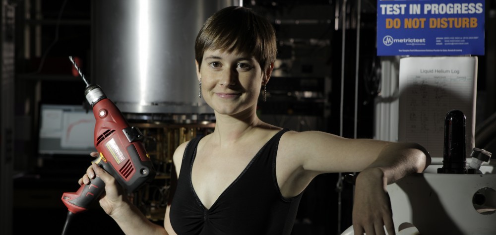
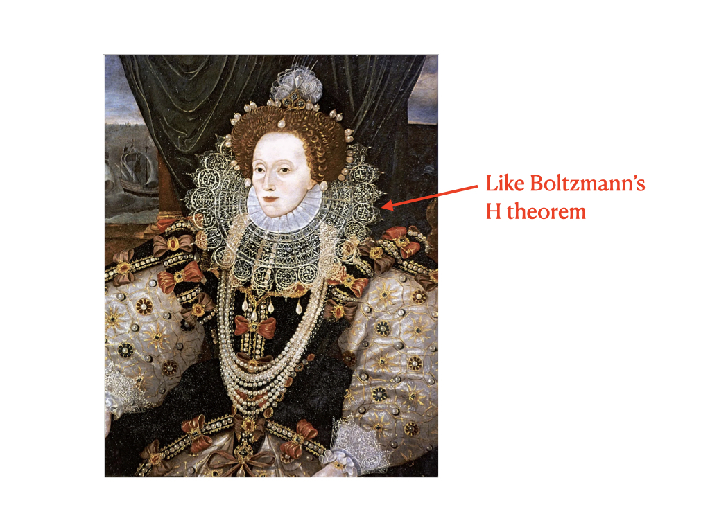
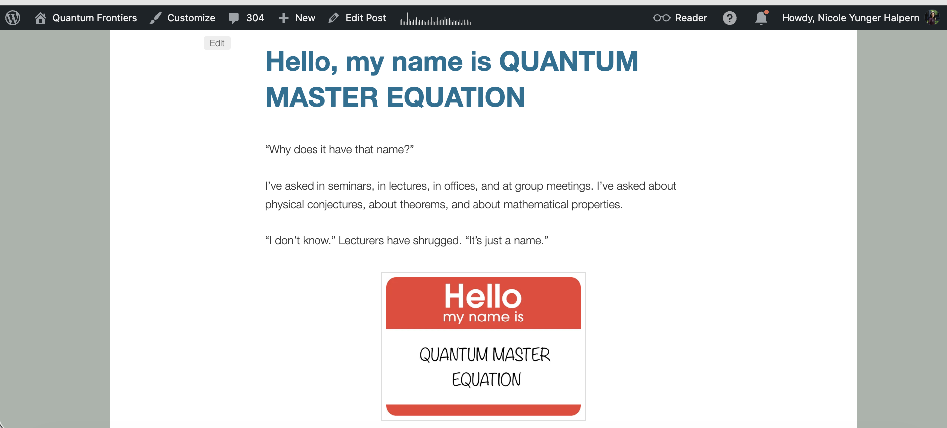
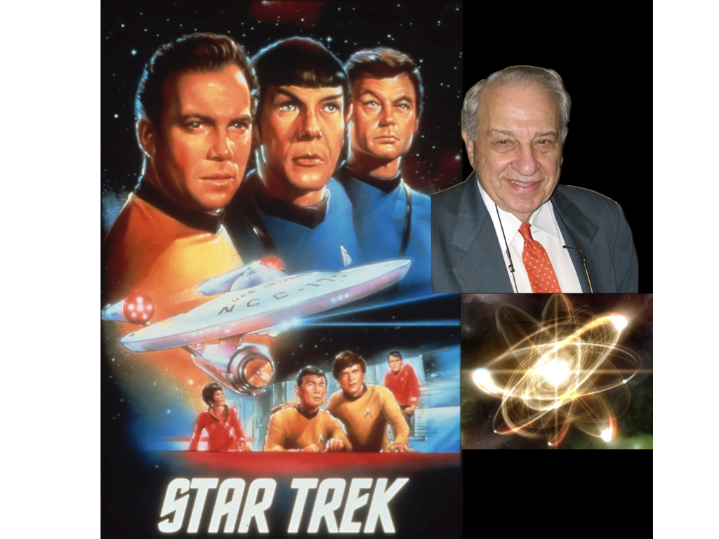

 means “greater than”; and
  , “greater than or equal to.” Don’t translate
  and
and  .
. . Evolve it under
  …”).
…”). defines a regime, not a limit. The conditions
  and
and  define limits and are inequivalent to
  Then Y.”
 then Y.
 . Substituting into Eq. (1) yields [equation].
 ,
, 
 denote the measurement outcome.
 denote the Pauli-
 operator of qubit
 :
:
 , encoding directionality.
 -axis
-axis , which means
  to physicists. Use
  instead, unless you’re writing for engineers (who denote
  (\ell) instead.
 , –,
, –,  , or
, or  . Find the symbol immediately rightward of the initial = sign. Begin the new line directly below that symbol.
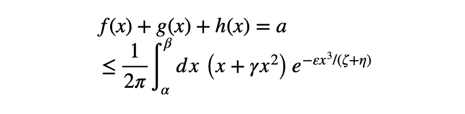
 in the example under (A). Put the corresponding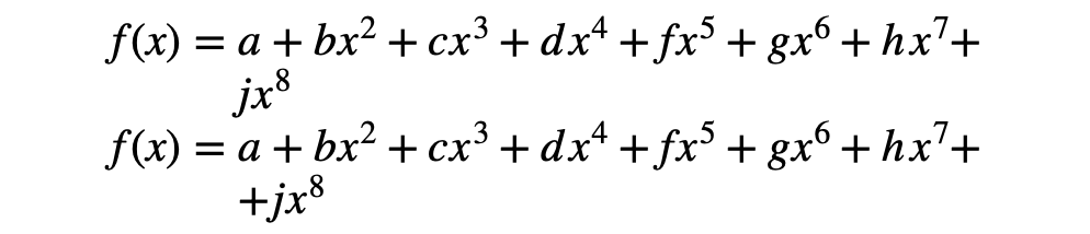
 means “approximately equals”; and ~, “scales as.” Approximations convey more information than scaling relations do.
 For example, if
  is odd, then
  and
and  fit the template.
 isn’t a matrix; a matrix represents an operator in terms of a particular basis. Therefore, no equals sign should interrelate an

 of real numbers
 and
and