A scientist in Florence can’t avoid bumping into colleagues.
When visiting the Renaissance’s birthplace last summer, I ran into a fellow physicist even on a Saturday morning. I was wandering around the Uffizi Gallery, a museum blessed with some of the greatest hits in western art. A familiar face arrested me on the first floor.
Another colleague cropped up outside the museum. (Some might classify him as an applied physicist or an engineer, but he exhibited a theoretical physicist’s overactive imagination.)
One colleague, I’d been looking forward to meeting for over four years. Jae Dong Noh is a professor of physics at the University of Seoul in South Korea. He’d conducted the first numerical tests (classical-computer simulations) of an idea I’d helped midwife, the non-Abelian eigenstate thermalization hypothesis (NAETH). An earlier blog post described this mouthful, which predicts how certain quantum many-particle systems thermalize, or experience the flow of time. These systems’ dynamics conserve properties, analogous to energy, that are incompatible: one can’t measure the properties simultaneously, as one can’t measure a quantum particle’s position and momentum simultaneously. Because incompatibility helps distinguish quantum from classical physics, such systems’ thermodynamics qualifies as particularly quantum.
Jae Dong modeled such a system and others numerically in a paper. I admired his computational techniques and his grasp of symmetries (for experts: how non-Abelian symmetries affect chaotic quantum systems’ energy-level statistics). My postdoc Aleks Lasek was planning a more thorough numerical test of the NAETH, so I reached out to Jae Dong, and a collaboration crystallized.
Seoul operates thirteen hours ahead of Maryland, but we managed to Zoom because Jae Dong is a night owl and I’m an early bird.1 Zoom introduced me to a man perpetually dressed in a neat button-down shirt and sweater, silver overriding the black in his hair. The neatness extended to Jae Dong’s explanations: if Aleks and I didn’t understand one of his emails, he’d explain it quietly and calmly, untangling the confusion as though pulling a comb through wool.
The collaboration settled into a rhythm: I’d pose a question or propose a goal, Jae Dong would respond with an analytical calculation,2 I’d find holes in the calculation, Jae Dong would plug the holes, I’d re-check the argument’s logic, and we’d repeat the cycle. Had I been in Jae Dong’s shoes, I’d have swallowed the constant objections as I’ve swallowed grape-flavored cough medicine,3 but he always responded with equanimity—sometimes even good cheer—and a possible solution. Meanwhile, Aleks and then-undergraduate Jade LeSchack checked our analytical arguments numerically.
Florence flaunted a little steampunk during my visit.
So smoothly did the collaboration hum along that we coauthored two papers before ever meeting in person. One demonstrates numerically that two quantum many-body systems (for experts: nonintegrable Heisenberg models) obey the NAETH.4 In the other paper, we derive a symmetry relation from the NAETH. If the 17-syllable NAETH is a mouthful, the symmetry’s name is half a mouthful: a Kubo–Martin–Schwinger (KMS) relation. It’s important because (i) it enables us to calculate how rapidly a thermodynamic system responds to a stimulus, such as a weak magnetic field, and (ii) physicists go gaga over symmetries generally.
The KMS relation constrains thermal states—essentially, systems that have temperatures. Your typical isolated many-particle quantum system looks thermal if you can observe just a small chunk of it at a time. Accordingly, Jae Dong and collaborators had proved that isolated many-particle quantum systems obey the KMS relation approximately. The larger the system, the more accurate the approximation.
We extended his argument to systems whose dynamics conserve incompatible properties. Such an extension might sound simple, but its proof filled 24 pages of appendices. (For experts: Clebsch–Gordan coefficients are tricky blighters.) We discovered that, under certain conditions, incompatible conserved quantities can reduce the extent to which a quantum system obeys the KMS relation. Quantum incompatibility can augment deviations from conventional thermodynamics.
Italy’s architecture impressed me.
Jae Dong planned to present about our work at StatPhys, an international statistical-physics conference, which Florence was hosting in 2024. Throughout the two-and-a-half months before the conference, the KMS relation consumed our team. (For experts: Clebsch–Gordan coefficients are very tricky blighters.) I even hid in my hotel room, working and reworking our proofs, during another conference during that time.
The toil paid off. We submitted our KMS manuscript for public scrutiny the day I flew to Florence—because not only Jae Dong would be representing our team at StatPhys. I was looking forward to meeting him there for the first time.
A corner of the hall where the StatPhys opening ceremony took place.
The StatPhys committee outdid itself. The opening ceremony unfolded in Florence’s Palazzo Vecchio, where members of the Medici dynasty once lived. Giorgio Parisi, who won a Nobel Prize for statistical physics in 2021, lectured at the ceremony.
Giorgio Parisi, with another history maker.
The meat of the conference took place in two other palaces, the Palazzo dei Congressi and the Palazzo degli Affari. In one of them, I met Jae Dong. Although we’d shown that quantum incompatibility can defy thermodynamic predictions, he met my expectations.
We discovered another thermodynamic phenomenon challenged by incompatible conserved quantities, so stay tuned for another paper and blog post. Some colleagues, one can’t avoid; others are worth engaging with again and again.
1 Aleks has confessed to night-owl habits, but physics motivates him to adapt. Some days, he’s emailed me results before even I’ve woken up. Who needs coffee when the thrill of discovery electrifies one minutes after one hops out of bed?
2 An exact calculation written out on paper, as opposed to a numerical, or approximate, calculation performed by a silicon-based classical computer.
3 Does anyone like the grape flavor? Why do companies bother producing it?
When I was pursuing a PhD at Caltech, so was my friend Jeremy. He used to throw a dinner party every few months. The email invitations welcomed friends to partake of his cooking and, if we wished, to help him cook. I didn’t help cook; but, when I arrived, the mess of pots and pans drew me to the kitchen like vinegar drawing a pathological fly. I couldn’t sit still while cookware needed cleaning, so I scrubbed and rinsed the pans and spoons and bowls. Jeremy, an applied-physics student, commented on my adeptness at decreasing entropy.
It’s the story of my life, I replied.
In fourth grade, my classmates and I cleaned our desks every Friday afternoon. Once a student finished, my teacher dismissed him or her onto the playground. My neighbor’s desk horrified me like the disaster in a hurricane’s wake, so I neatened his desk after finishing with mine.1 Another friend requested the same favor. A third classmate offered to pay me for cleaning his desk, but I’d have undertaken the chore for its own sake. Ordering the world offered me fulfillment.
From cleaning a fourth-grade desk, I progressed to pursuing a PhD in theoretical physics. The two pursuits might seem to resemble each other no more than Dr. Jekyll and Mr. Hyde; yet, to me, the path between them is but a step. I trained as a theoretical physicist because I love organizing ideas. Caltech paid me to build models, propose definitions and theorems, and structure proofs—to dream up ideas and identify the optimal arrangements for them. I needed that pay, being an adult, as I hadn’t needed my fourth-grade classmate’s desk-cleaning fee. Yet I organized ideas for the same reason that drove me to organize my neighbor’s notebooks.
Many people have called entropy a measure of disorder. To see why, imagine that Jeremy’s crew has used thirty utensils while cooking. The chefs can have scattered the utensils across the kitchen in many ways: they may have dropped forks on the floor, left spoons in the sink, arranged spatulas on the drying rack, or filled a vase with knives like a modern-art bouquet. In few of these configurations do the forks lie in their compartment of the utensil drawer, the spoons lie in their compartment, etc. We call such configurations neat. Most of the other configurations, we call messy.
A system’s entropy is the number of configurations consistent with known large-scale properties of the system, such as the number of forks.2 More configurations are consistent with messiness (and a fixed number of forks and so on) than with neatness (and the same number of forks and so on). Messiness tends to correlate with high entropy. People often say, therefore, that entropy quantifies messiness. Hence Jeremy’s complimenting me on my decreasing of entropy.
Jeremy’s dinner parties came to mind as I read the book The Mattering Instinct, published by Rebecca Newberger Goldstein this January. Rebecca is a philosopher of science and a writer. I had the good fortune to meet her through my undergraduate mentor Marcelo Gleiser, who’s had another cameo or two on Quantum Frontiers. Rebecca’s latest book covers what she calls the mattering instinct: the longing to know that we matter.
We spend scads of energy and time on securing our “survival and flourishing,” as Rebecca says. We feed ourselves; work to earn money to purchase food; clean, shelter, and clothe ourselves; ingrain ourselves in societies that offer some degree of security; and more. Do we deserve all this effort? We long for assurance that, in the immortal words of L’Oreal, we’re worth it.
Survival and flourishing, Rebecca writes, requires us to decrease entropy. Every closed, isolated system’s entropy increases or remains constant, according to the second law of thermodynamics. Entropy increases as a system becomes more uniform, loosely speaking. The system’s particles spread out across space, these particles’ temperature comes to equal those particles’ temperature, and so on. In contrast, your body exists because its particles clump together in a certain shape consistently. You withstand heat waves and snow because homeostasis maintains your temperature despite your environment’s temperature. You keep your body’s entropy low to survive. Rebecca therefore casts us as fighting entropy.
As a thermodynamicist, I agree with Rebecca. Yet I also adore entropy. It helps explain why time flows, quantifies uncertainty, and determines the maximal efficiencies with which we can perform tasks such as communication. What versatility and richness! Entropy also embodies tension and subtlety: its mathematical definition looks obscure at first glance, yet entropy helps explain familiar phenomena such as aging. For these reasons, before beginning my PhD, I told a potential advisor that I could imagine devoting the next five years of my life to entropy.
I therefore aspire to rehabilitate entropy’s reputation. Novelist Terry Pratchett endeared mortality to millions of readers through anthropomorphism. His character Death, a mainstay of the Discworld series of novels, elicits empathy and fondness. I won’t anthropomorphize entropy here,3 but I aim to replace conflict with cooperation in the narrative above. To survive and flourish, I hold, we partner with entropy. How? We create oodles of entropy in our environments. This entropy increase offsets the entropy decrease that supports life.
For example, imagine working at a desalination plant. You’d process high-entropy water throughout which salt has spread. You’d concentrate the salt in a tiny region, reducing the water’s entropy. This reduction, producing fresh water, could support your city’s drinking, cooking, and toothbrushing needs.
To reduce the water’s entropy, you’d create loads more entropy. You’d eat breakfast before work, consuming energy stored neatly in your waffle’s chemical bonds. Your body would later break the bonds, releasing the energy. Some energy would power your muscles, so you could program the desalination system, test its output, etc. But much of the chemical energy would transform into heat radiated by your body. The heat would warm up the air molecules around you, magnifying their random jigglings and jostlings. You’d increase the entropy of the air—your environment—to decrease the water’s entropy. The air’s entropy increase would outweigh the water’s entropy decrease.
Organisms survive and flourish by producing entropy in their environments. In fact, organisms have a knack for generating entropy. Entropy and life thereby further each other. A glass-half-full thinker could conclude that we partner with entropy.
So did I partner with entropy as a PhD student, applying it to solve problems in quantum information theory and thermodynamics. So did I partner with entropy in fourth grade and at Jeremy’s apartment, deriving satisfaction from my cleaning. Rebecca would call these activities’ ultimate aim (beyond the aim of, e.g., not sitting beside a pigsty in fourth grade) mattering. She writes that we reduce entropy (within our immediate vicinities) to satisfy the mattering instinct. Rebecca’s proposition describes my behaviors with uncanny precision, I realized upon reading her book.
Which I’ve now finished. So pardon me while I return to washing forks in the quantum kitchen of the universe.
With thanks to Jeremy for his friendship…and food.
1I also ensured that my neighbor brought home, every afternoon, the sweater he’d brought to school that morning. Before I took charge, he’d ended up with three forgotten sweaters crammed into his cubby.
As experimental capabilities advance rapidly, the quantum computing community faces a critical elephant in the room: What will these quantum machines eventually be useful for? Will they deliver the promised broad societal impact, or will they remain highly specialized devices for exotic tasks known only to the experts?
The elephant in the room
Despite decades of effort, conclusive evidence of large quantum advantage in real-world applications remains confined to a few niche domains, such as simulating quantum materials and cryptanalysis. These problems are either inherently quantum to begin with, or they possess specialized mathematical structure that quantum algorithms can easily exploit. But it seems unlikely that such structures appear broadly in everyday life.
Indeed, most applications of modern computation hinge on the processing of massive, noisy classical data, generated at an unprecedented pace across society. That is the driving force behind the overwhelming success of machine learning and AI. Since the data originates from the macroscopic classical world, there is no obvious reason it should exhibit the delicate, specialized structures that quantum computers require. To playfully adapt Richard Feynman’s famous quote: We live in an effectively classical world, dammit, and maybe classical computers and AI already suffice for most of our problems. (For those unfamiliar, Feynman originally quipped: “Nature isn’t classical, dammit, and if you want to make a simulation of nature, you’d better make it quantum mechanical.”)
The central challenge
To truly unlock the power of a quantum computer, quantum algorithms typically need to access data in quantum superposition, processing many different samples simultaneously in different branches of the quantum multiverse. To use technical jargon, this is called querying a quantum oracle. But in reality, the classical data samples that we want to process are generated from everyday activities in a classical world, and we can only access them one at a time.
Think of the movie reviews you scroll through on a streaming platform. How would you read the plain-text reviews from a million different users all at once in a quantum superposition? This bottleneck—the challenge of efficiently accessing the classical world in quantum superposition—is known as the data loading problem. It has arguably been one of the main obstacles to achieving broadly applicable quantum advantage.
Sketching a quantum oracle
In this new work [1], we provide a solution to this seemingly impossible challenge. We develop a framework, called quantum oracle sketching, that enables us to access the classical world in quantum superposition in an optimal way. Importantly, it automatically handles the noise and correlations in the data, and natively supports flexible data structures like vectors and matrices that enable machine learning applications.
The core mechanism relies on processing data as a continuous stream. For each classical data sample we observe, we apply a carefully designed, small quantum rotation to our system. By sequentially accumulating these quantum rotations, we incrementally build up an accurate approximation of the target quantum oracle, which can then be used in any quantum algorithm for data processing. Because every data sample is processed once and immediately discarded, we completely eliminate the massive memory overhead typically required to store the dataset. The fundamental price to pay for assembling quantum queries from classical data lies in the sample complexity: our algorithm consumes a number of samples that scales quadratically with the number of quantum queries we need to make. We show that this rate is optimal and fundamentally arises from the quadratic relationship between quantum amplitudes and classical probabilities governed by the Born rule.
With the data successfully loaded into the quantum computer, the final challenge is to efficiently read out classical results. To address this, we develop an efficient measurement protocol called interferometric classical shadow. Combined with quantum oracle sketching, it allows us to circumvent the data loading and readout bottleneck to construct exponentially compact classical models from massive classical data with quantum technology.
Exponential quantum advantage in machine learning
Using this new approach, we are finally able to find exponential quantum advantage in processing classical data and machine learning. We rigorously prove that a small quantum computer can perform large-scale classification and dimensionality reduction on massive classical data by processing samples on the fly. In contrast, any classical machine achieving the same prediction performance requires exponentially larger size. When the classical machine does not have the required exponentially large memory size, it needs super-polynomially more samples and time relative to our protocol running on a quantum device. Remarkably, this illustrates that quantum technology enables us to construct compact and accurate classical models out of classical data, which is impossible with classical machines alone unless given exponentially larger memory.
The true scale of this exponential memory advantage is staggering. A quantum processor with 300 logical qubits can outperform a classical machine built from every atom in the observable universe. Of course, to actually see such a comical contrast, we would also need universe-scale datasets and processing time.
To contextualize these results in realistic scenarios, consider a large-scale scientific experiment, like a large particle collider. Each experimental run generates a colossal volume of data. With a quantum computer, we can keep squeezing all the data into this tiny quantum chip to perform downstream machine learning tasks such as classification and dimensionality reduction. But if we only have classical machines, we would need to build massive, energy-consuming data centers to store the raw data to match the performance. Without this massive memory overhead, classical machines simply couldn’t extract the same clear signals from a single run, forcing us to repeat the massive, expensive experiment many more times to compensate. To put this into perspective, the Large Hadron Collider (LHC) at CERN generates petabytes (millions of gigabytes) of data per hour, but the data storage bottlenecks force researchers to discard all but a tiny fraction—retaining perhaps only one in a hundred thousand events.
We validated these quantum advantages on real-world datasets, including movie review sentiment analysis and single-cell RNA sequencing. In these public datasets, we demonstrate four to six orders of magnitude (ten thousand to a million times) reduction in memory size with fewer than 60 logical qubits. Given the rapid advancements in high-rate quantum error correction codes and experimental techniques, quantum computers capable of demonstrating such applications are foreseeable in the near future. Crucially, the quantum advantage we propose likely carries a clearer positive impact for society and likely arrives sooner than the applications in cryptanalysis, where the current best estimate requires a thousand logical qubits.
Towards Quantum AI
Our results provide strong evidence that the utility of quantum computers extends far beyond specialized tasks, opening a path for quantum computers to be broadly useful in our everyday life. Rather than fearing that classical AI will “eat quantum computing’s lunch,” we now have rigorous evidence pointing towards a much more exciting prospect: quantum-enhanced AI overpowering classical AI.
Of course, there is still a long way to go towards the dream of quantum intelligence. Our current results establish the provable supremacy of quantum machines in foundational machine learning tasks, such as high-dimensional linear classification and dimensionality reduction. They do not yet imply immediate utility for modern generative AI such as large language models.
That said, our results give me a strong feeling that we are living in an age strikingly reminiscent of the traditional machine learning era—an age dominated by support vector machines and random forests; an age when we relied on rigorous statistical analysis because we lacked the computational resources for large-scale heuristic exploration; an age that ultimately heralded the birth of deep learning and the AI revolution. Today, quantum AI seems to sit at a similar historical position. I cannot wait to see what quantum AI will become once we are capable of unconstrained heuristic exploration on large-scale fault-tolerant quantum computers.
To accelerate this dawn of quantum AI, we invite physicists, computer scientists, developers, and machine learning practitioners to join our efforts and help us push the boundaries of what quantum AI can achieve. To bridge the gap between abstract quantum theory and hands-on machine learning practice, we are open-sourcing our core framework. Our numerical implementation of quantum oracle sketching is built in JAX, natively supporting GPU/TPU acceleration and automatic differentiation to integrate nicely with modern machine learning pipelines. Check out the code, run the simulations, and help us shape the future of quantum AI at github.com/haimengzhao/quantum-oracle-sketching!
My top 10 ghosts (solo acts and ensembles). If Bruce Willis being a ghost in The Sixth Sense is a spoiler, that’s on you — the movie has been out for 26 years.
Einstein and I have both been spooked by entanglement. Einstein’s experience was more profound: in a 1947 letter to Born, he famously dubbed it spukhafte Fernwirkung (or spooky action at a distance). Mine, more pedestrian. It came when I first learned the cost of entangling logical qubits on today’s hardware.
Logical entanglement is not easy
I recently listened to a talk where the speaker declared that “logical entanglement is easy,” and I have to disagree. You could argue that it looks easy when compared to logical small-angle gates, in much the same way I would look small standing next to Shaquille O’Neal. But that doesn’t mean 6’5” and 240 pounds is small.
To see why it’s not easy, it helps to look at how logical entangling gates are actually implemented. A logical qubit is not a single physical object. It’s an error-resistant qubit built out of several noisy, error-prone physical qubits. A quantum error-correcting (QEC) code with parameters uses physical qubits to encode logical qubits in a way that can detect up to physical errors and correct up to of them.
This redundancy is what makes fault-tolerant quantum computing possible. It’s also what makes logical operations expensive.
On platforms like neutral-atom arrays and trapped ions, the standard approach is a transversal CNOT: you apply two-qubit gates pairwise across the code blocks (qubit in block A interacts with qubit in block B). That requires physical two-qubit gates to entangle the logical qubits of one code block with the logical qubits of another.
To make this less abstract, here’s a QuEra animation showing a transversal CNOT implemented in a neutral-atom array. This animation is showing real experimental data, not a schematic idealization.
The idea is simple. The problem is that can be large, and physical two-qubit gates are among the noisiest operations available on today’s hardware.
Superconducting platforms take a different route. They tend to rely on lattice surgery; you entangle logical qubits by repeatedly measuring joint stabilizers along a boundary. That replaces two-qubit gates for stabilizer measurements over multiple rounds (typically scaling with the code distance). Unfortunately, physical measurements are the other noisiest primitive we have.
Then there are the modern high-rate qLDPC codes, which pack many logical qubits into a single code block. These are excellent quantum memories. But when it comes to computation, they face challenges. Logical entangling gates can require significant circuit depth, and often entire auxiliary code blocks are needed to mediate the interaction.
This isn’t a purely theoretical complaint. In recent state-of-the-art experiments by Google and by the Harvard–QuEra–MIT collaboration, logical entangling gates consumed nearly half of the total error budget.
So no, logical entanglement is not easy. But, how easy can we make it?
Phantom codes: Logical entanglement without physical operations
To answer how easy logical entanglement can really be, it helps to start with a slightly counterintuitive observation: logical entanglement can sometimes be generated purely by permuting physical qubits.
Let me show you how this works in the simplest possible setting, and then I’ll explain what’s really going on.
Consider a stabilizer code, which encodes 4 physical qubits into 2 logical ones that can detect 1 error, but can’t correct any. Below are its logical operators; the arrow indicates what happens when we physically swap qubits 1 and 3 (bars denote logical operators).
You can check that the logical operators transform exactly as shown, which is the action of a logical CNOT gate. For readers less familiar with stabilizer codes, click the arrow below for an explanation of what’s going on. Those familiar can carry on.
Click!
At the logical level, we identify gates by how they transform logical Pauli operators. This is the same idea used in ordinary quantum circuits: a gate is defined not just by what it does to states, but by how it reshuffles observables.
A CNOT gate has a very characteristic action. If qubit 1 is the control and qubit 2 is the target, then: an on the control spreads to the target, a on the target spreads back to the control, and the other Pauli operators remain unchanged.
That’s exactly what we see above.
To see why this generates entanglement, it helps to switch from operators to states. A canonical example of how to generate entanglement in quantum circuits is the following. First, you put one qubit into a superposition using a Hadamard. Starting from , this gives
At this point there is still no entanglement — just superposition.
The entanglement appears when you apply a CNOT. The CNOT correlates the two branches of the superposition, producing
which is a maximally-entangled Bell state. The Hadamard creates superposition; the CNOT turns that superposition into correlation.
The operator transformations above are simply the algebraic version of this story. Seeing
tells us that information on one logical qubit is now inseparable from the other.
In other words, in this code,
The figure below shows how this logical circuit maps onto a physical circuit. Each horizontal line represents a qubit. On the left is a logical CNOT gate: the filled dot marks the control qubit, and the ⊕ symbol marks the target qubit whose state is flipped if the control is in the state . On the right is the corresponding physical implementation, where the logical gate is realized by acting on multiple physical qubits.
At this point, all we’ve done is trade one physical operation for another. The real magic comes next. Physical permutations do not actually need to be implemented in hardware. Because they commute cleanly through arbitrary circuits, they can be pulled to the very end of a computation and absorbed into a relabelling of the final measurement outcomes. No operator spread. No increase in circuit depth.
This is not true for generic physical gates. It is a unique property of permutations.
To see how this works, consider a slightly larger example using an code. Here the logical operators are a bit more complicated:
Below is a three-logical-qubit circuit implemented using this code like the circuit drawn above, but now with an extra step. Suppose the circuit contains three logical CNOTs, each implemented via a physical permutation.
Instead of executing any of these permutations, we simply keep track of them classically and relabel the outputs at the end. From the hardware’s point of view, nothing happened.
If you prefer a more physical picture, imagine this implemented with atoms in an array. The atoms never move. No gates fire. The entanglement is there anyway.
This is the key point. Because no physical gates are applied, the logical entangling operation has zero overhead. And for the same reason, it has perfect fidelity. We’ve reached the minimum possible cost of a logical entangling gate. You can’t beat free.
To be clear, not all codes are amenable to logical entanglement through relabeling. This is a very special feature that exists in some codes.
Motivated by this observation, my collaborators and I defined a new class of QEC codes. I’ll state the definition first, and then unpack what it really means.
Phantom codes are stabilizer codes in which logical entangling gates between every ordered pair of logical qubits can be implemented solely via physical qubit permutations.
The phrase “every ordered pair” is a strong requirement. For three logical qubits, it means the code must support logical CNOTs between qubits , , , , , and . More generally, a code with logical qubits must support all possible directed CNOTs. This isn’t pedantry. Without access to every directed pair, you can’t freely build arbitrary entangling circuits — you’re stuck with a restricted gate set.
The phrase “solely via physical qubit permutations” is just as demanding. If all but one of those CNOTs could be implemented via permutations, but the last one required even a single physical gate — say, a one-qubit Clifford — the code would not be phantom. That condition is what buys you zero overhead and perfect fidelity. Permutations can be compiled away entirely; any additional physical operation cannot.
Together, these two requirements carve out a very special class of codes. All in-block logical entangling gates are free. Logical entangling gates between phantom code blocks are still available — they’re simply implemented transversally.
After settling on this definition, we went back through the literature to see whether any existing codes already satisfied it. We found two. The Carbon code and hypercube codes. The former enabled repeated rounds of quantum error-correction in trapped-ion experiments, while the latter underpinned recent neutral-atom experiments achieving logical-over-physical performance gains in quantum circuit sampling.
Both are genuine phantom codes. Both are also limited. With distance , they can detect errors but not correct them. With only logical qubits, there’s a limited class of CNOT circuits you can implement. Which begs the questions: Do other phantom codes exist? Can these codes have advantages that persist for scalable applications under realistic noise conditions? What structural constraints do they obey (parameters, other gates, etc.)?
Before getting to that, a brief note for the even more expert reader on four things phantom codes are not. Phantom codes are not a form of logical Pauli-frame tracking: the phantom property survives in the presence of non-Clifford gates. They are not strictly confined to a single code block: because they are CSS codes, multiple blocks can be stitched together using physical CNOTs in linear depth. They are not automorphism gates, which rely on single-qubit Cliffords and therefore do not achieve zero overhead or perfect fidelity. And they are not codes like SHYPS, Gross, or Tesseract codes, which allow only products of CNOTs via permutations rather than individually addressable ones. All of those codes are interesting. They’re just not phantom codes.
In a recent preprint, we set out to answer the three questions above. This post isn’t about walking through all of those results in detail, so here’s the short version. First, we find many more phantom codes — hundreds of thousands of additional examples, along with infinite families that allow both and to scale. We study their structural properties and identify which other logical gates they support beyond their characteristic phantom ones.
Second, we show that phantom codes can be practically useful for the right kinds of tasks — essentially, those that are heavy on entangling gates. In end-to-end noisy simulations, we find that phantom codes can outperform the surface code, achieving one–to–two orders of magnitude reductions in logical infidelity for resource state preparation (GHZ-state preparation) and many-body simulation, at comparable qubit overhead and with a modest preselection acceptance rate of about 24%.
If you’re interested in the details, you can read more in our preprint.
Larger space of codes to explore
This is probably a good moment to zoom out and ask the referee question: why does this matter?
I was recently updating my CV and realized I’ve now written my 40th referee report for APS. After a while, refereeing trains a reflex. No matter how clever the construction or how clean the proof, you keep coming back to the same question: what does this actually change?
So why do phantom codes matter? At least to me, there are two reasons: one about how we think about QEC code design, and one about what these codes can already do in practice.
The first reason is the one I’m most excited about. It has less to do with any particular code and more to do with how the field implicitly organizes the space of QEC codes. Most of that space is structured around familiar structural properties: encoding rate, distance, stabilizer weight, LDPC-ness. These form the axes that make a code a good memory. And they matter, a lot.
But computation lives on a different axis. Logical gates cost something, and that cost is sometimes treated as downstream—something to be optimized after a code is chosen, rather than something to design for directly. As a result, the cost of logical operations is usually inherited, not engineered.
One way to make this tension explicit is to think of code design as a multi-dimensional space with at least two axes. One axis is memory cost: how efficiently a code stores information. High rate, high distance, low-weight stabilizers, efficient decoding — all the usual virtues. The other axis is computational cost: how expensive it is to actually do things with the encoded qubits. Low computational cost means many logical gates can be implemented with little overhead. Low computational cost makes computation easy.
Why focus on extreme points in this space? Because extremes are informative. They tell you what is possible, what is impossible, and which tradeoffs are structural rather than accidental.
Phantom codes sit precisely at one such extreme: they minimize the cost of in-block logical entanglement. That zero-logical-cost extreme comes with tradeoffs. The phantom codes we find tend to have high stabilizer weights, and for families with scalable , the number of physical qubits grows exponentially. These are real costs, and they matter.
Still, the important lesson is that even at this extreme point, codes can outperform LDPC-based architectures on well-chosen tasks. That observation motivates an approach to QEC code design in which the logical gates of interest are placed at the centre of the design process, rather than treated as an afterthought. This is my first takeaway from this work.
Second is that phantom codes are naturally well suited to circuits that are heavy on logical entangling gates. Some interesting applications fall into this category, including fermionic simulation and correlated-phase preparation. Combined with recent algorithmic advances that reduce the overhead of digital fermionic simulation, these code-level ideas could potentially improve near-term experimental feasibility.
Back to being spooked
The space of QEC codes is massive. Perhaps two axes are not enough. Stabilizer weight might deserve its own. Perhaps different applications demand different projections of this space. I don’t yet know the best way to organize it.
The size of this space is a little spooky — and that’s part of what makes it exciting to explore, and to see what these corners of code space can teach us about fault-tolerant quantum computation.
On December 10, I gave a keynote address at the Q2B 2025 Conference in Silicon Valley. This is a transcript of my remarks. The slides I presented are here.The video is here.
The first century
We are nearing the end of the International Year of Quantum Science and Technology, so designated to commemorate the 100th anniversary of the discovery of quantum mechanics in 1925. The story goes that 23-year-old Werner Heisenberg, seeking relief from severe hay fever, sailed to the remote North Sea Island of Helgoland, where a crucial insight led to his first, and notoriously obscure, paper describing the framework of quantum mechanics.
In the years following, that framework was clarified and extended by Heisenberg and others. Notably among them was Paul Dirac, who emphasized that we have a theory of almost everything that matters in everyday life. It’s the Schrödinger equation, which captures the quantum behavior of many electrons interacting electromagnetically with one another and with atomic nuclei. That describes everything in chemistry and materials science and all that is built on those foundations. But, as Dirac lamented, in general the equation is too complicated to solve for more than a few electrons.
Somehow, over 50 years passed before Richard Feynman proposed that if we want a machine to help us solve quantum problems, it should be a quantum machine, not a classical machine. The quest for such a machine, he observed, is “a wonderful problem because it doesn’t look so easy,” a statement that still rings true.
I was drawn into that quest about 30 years ago. It was an exciting time. Efficient quantum algorithms for the factoring and discrete log problems were discovered, followed rapidly by the first quantum error-correcting codes and the foundations of fault-tolerant quantum computing. By late 1996, it was firmly established that a noisy quantum computer could simulate an ideal quantum computer efficiently if the noise is not too strong or strongly correlated. Many of us were then convinced that powerful fault-tolerant quantum computers could eventually be built and operated.
Three decades later, as we enter the second century of quantum mechanics, how far have we come? Today’s quantum devices can perform some tasks beyond the reach of the most powerful existing conventional supercomputers. Error correction had for decades been a playground for theorists; now informative demonstrations are achievable on quantum platforms. And the world is investing heavily in advancing the technology further.
Current NISQ machines can perform quantum computations with thousands of two-qubit gates, enabling early explorations of highly entangled quantum matter, but still with limited commercial value. To unlock a wide variety of scientific and commercial applications, we need machines capable of performing billions or trillions of two-qubit gates. Quantum error correction is the way to get there.
I’ll highlight some notable developments over the past year—among many others I won’t have time to discuss. (1) We’re seeing intriguing quantum simulations of quantum dynamics in regimes that are arguably beyond the reach of classical simulations. (2) Atomic processors, both ion traps and neutral atoms in optical tweezers, are advancing impressively. (3) We’re acquiring a deeper appreciation of the advantages of nonlocal connectivity in fault-tolerant protocols. (4) And resource estimates for cryptanalytically relevant quantum algorithms have dropped sharply.
Quantum machines for science
A few years ago, I was not particularly excited about running applications on the quantum platforms that were then available; now I’m more interested. We have superconducting devices from IBM and Google with over 100 qubits and two-qubit error rates approaching 10^{-3}. The Quantinuum ion trap device has even better fidelity as well as higher connectivity. Neutral-atom processors have many qubits; they lag behind now in fidelity, but are improving.
Users face tradeoffs: The high connectivity and fidelity of ion traps is an advantage, but their clock speeds are orders of magnitude slower than for superconducting processors. That limits the number of times you can run a given circuit, and therefore the attainable statistical accuracy when estimating expectations of observables.
Verifiable quantum advantage
Much attention has been paid to sampling from the output of random quantum circuits, because this task is provably hard classically under reasonable assumptions. The trouble is that, in the high-complexity regime where a quantum computer can reach far beyond what classical computers can do, the accuracy of the quantum computation cannot be checked efficiently. Therefore, attention is now shifting toward verifiable quantum advantage — tasks where the answer can be checked. If we solved a factoring or discrete log problem, we could easily check the quantum computer’s output with a classical computation, but we’re not yet able to run these quantum algorithms in the classically hard regime. We might settle instead for quantum verification, meaning that we check the result by comparing two quantum computations and verifying the consistency of the results.
A type of classical verification of a quantum circuit was demonstrated recently by BlueQubit on a Quantinuum processor. In this scheme, a designer builds a family of so-called “peaked” quantum circuits such that, for each such circuit and for a specific input, one output string occurs with unusually high probability. An agent with a quantum computer who knows the circuit and the right input can easily identify the preferred output string by running the circuit a few times. But the quantum circuits are cleverly designed to hide the peaked output from a classical agent — one may argue heuristically that the classical agent, who has a description of the circuit and the right input, will find it hard to predict the preferred output. Thus quantum agents, but not classical agents, can convince the circuit designer that they have reliable quantum computers. This observation provides a convenient way to benchmark quantum computers that operate in the classically hard regime.
The notion of quantum verification was explored by the Google team using Willow. One can execute a quantum circuit acting on a specified input, and then measure a specified observable in the output. By repeating the procedure sufficiently many times, one obtains an accurate estimate of the expectation value of that output observable. This value can be checked by any other sufficiently capable quantum computer that runs the same circuit. If the circuit is strategically chosen, then the output value may be very sensitive to many-qubit interference phenomena, in which case one may argue heuristically that accurate estimation of that output observable is a hard task for classical computers. These experiments, too, provide a tool for validating quantum processors in the classical hard regime. The Google team even suggests that such experiments may have practical utility for inferring molecular structure from nuclear magnetic resonance data.
Correlated fermions in two dimensions
Quantum simulations of fermionic systems are especially compelling, since electronic structure underlies chemistry and materials science. These systems can be hard to simulate in more than one dimension, particularly in parameter regimes where fermions are strongly correlated, or in other words profoundly entangled. The two-dimensional Fermi-Hubbard model is a simplified caricature of two-dimensional materials that exhibit high-temperature superconductivity and hence has been much studied in recent decades. Large-scale tensor-network simulations are reasonably successful at capturing static properties of this model, but the dynamical properties are more elusive.
Dynamics in the Fermi-Hubbard model has been simulated recently on both Quantinuum (here and here) and Google processors. Only a 6 x 6 lattice of electrons was simulated, but this is already well beyond the scope of exact classical simulation. Comparing (error-mitigated) quantum circuits with over 4000 two-qubit gates to heuristic classical tensor-network and Majorana path methods, discrepancies were noted, and the Phasecraft team argues that the quantum simulation results are more trustworthy. The Harvard group also simulated models of fermionic dynamics, but were limited to relatively low circuit depths due to atom loss. It’s encouraging that today’s quantum processors have reached this interesting two-dimensional strongly correlated regime, and with improved gate fidelity and noise mitigation we can go somewhat further, but expanding system size substantially in digital quantum simulation will require moving toward fault-tolerant implementations. We should also note that there are analog Fermi-Hubbard simulators with thousands of lattice sites, but digital simulators provide greater flexibility in the initial states we can prepare, the observables we can access, and the Hamiltonians we can reach.
When it comes to many-particle quantum simulation, a nagging question is: “Will AI eat quantum’s lunch?” There is surging interest in using classical artificial intelligence to solve quantum problems, and that seems promising. How will AI impact our quest for quantum advantage in this problem space? This question is part of a broader issue: classical methods for quantum chemistry and materials have been improving rapidly, largely because of better algorithms, not just greater processing power. But for now classical AI applied to strongly correlated matter is hampered by a paucity of training data. Data from quantum experiments and simulations will likely enhance the power of classical AI to predict properties of new molecules and materials. The practical impact of that predictive power is hard to clearly foresee.
The need for fundamental research
Today is December 10th, the anniversary of Alfred Nobel’s death. The Nobel Prize award ceremony in Stockholm concluded about an hour ago, and the Laureates are about to sit down for a well-deserved sumptuous banquet. That’s a fitting coda to this International Year of Quantum. It’s useful to be reminded that the foundations for today’s superconducting quantum processors were established by fundamental research 40 years ago into macroscopic quantum phenomena. No doubt fundamental curiosity-driven quantum research will continue to uncover unforeseen technological opportunities in the future, just as it has in the past.
I have emphasized superconducting, ion-trap, and neutral atom processors because those are most advanced today, but it’s vital to continue to pursue alternatives that could suddenly leap forward, and to be open to new hardware modalities that are not top-of-mind at present. It is striking that programmable, gate-based quantum circuits in neutral-atom optical-tweezer arrays were first demonstrated only a few years ago, yet that platform now appears especially promising for advancing fault-tolerant quantum computing. Policy makers should take note!
The joy of nonlocal connectivity
As the fault-tolerant era dawns, we increasingly recognize the potential advantages of the nonlocal connectivity resulting from atomic movement in ion traps and tweezer arrays, compared to geometrically local two-dimensional processing in solid-state devices. Over the past few years, many contributions from both industry and academia have clarified how this connectivity can reduce the overhead of fault-tolerant protocols.
Even when using the standard surface code, the ability to implement two-qubit logical gates transversally—rather than through lattice surgery—significantly reduces the number of syndrome-measurement rounds needed for reliable decoding, thereby lowering the time overhead of fault tolerance. Moreover, the global control and flexible qubit layout in tweezer arrays increase the parallelism available to logical circuits.
Nonlocal connectivity also enables the use of quantum low-density parity-check (qLDPC) codes with higher encoding rates, reducing the number of physical qubits needed per logical qubit for a target logical error rate. These codes now have acceptably high accuracy thresholds, practical decoders, and—thanks to rapid theoretical progress this year—emerging constructions for implementing universal logical gate sets. (See for example here, here, here, here.)
A serious drawback of tweezer arrays is their comparatively slow clock speed, limited by the timescales for atom transport and qubit readout. A millisecond-scale syndrome-measurement cycle is a major disadvantage relative to microsecond-scale cycles in some solid-state platforms. Nevertheless, the reductions in logical-gate overhead afforded by atomic movement can partially compensate for this limitation, and neutral-atom arrays with thousands of physical qubits already exist.
To realize the full potential of neutral-atom processors, further improvements are needed in gate fidelity and continuous atom loading to maintain large arrays during deep circuits. Encouragingly, active efforts on both fronts are making steady progress.
Approaching cryptanalytic relevance
Another noteworthy development this year was a significant improvement in the physical qubit count required to run a cryptanalytically relevant quantum algorithm, reduced by Gidney to less than 1 million physical qubits from the 20 million Gidney and Ekerå had estimated earlier. This applies under standard assumptions: a two-qubit error rate of 10^{-3} and 2D geometrically local processing. The improvement was achieved using three main tricks. One was using approximate residue arithmetic to reduce the number of logical qubits. (This also suppresses the success probability and therefore lengthens the time to solution by a factor of a few.) Another was using a more efficient scheme to reduce the number of physical qubits for each logical qubit in cold storage. And the third was a recently formulated scheme for reducing the spacetime cost of non-Clifford gates. Further cost reductions seem possible using advanced fault-tolerant constructions, highlighting the urgency of accelerating migration from vulnerable cryptosystems to post-quantum cryptography.
Looking forward
Over the next 5 years, we anticipate dramatic progress toward scalable fault-tolerant quantum computing, and scientific insights enabled by programmable quantum devices arriving at an accelerated pace. Looking further ahead, what might the future hold? I was intrigued by a 1945 letter from John von Neumann concerning the potential applications of fast electronic computers. After delineating some possible applications, von Neumann added: “Uses which are not, or not easily, predictable now, are likely to be the most important ones … they will … constitute the most surprising extension of our present sphere of action.” Not even a genius like von Neumann could foresee the digital revolution that lay ahead. Predicting the future course of quantum technology is even more hopeless because quantum information processing entails an even larger step beyond past experience.
As we contemplate the long-term trajectory of quantum science and technology, we are hampered by our limited imaginations. But one way to loosely characterize the difference between the past and the future of quantum science is this: For the first hundred years of quantum mechanics, we achieved great success at understanding the behavior of weakly correlated many-particle systems, leading for example to transformative semiconductor and laser technologies. The grand challenge and opportunity we face in the second quantum century is acquiring comparable insight into the complex behavior of highly entangled states of many particles, behavior well beyond the scope of current theory or computation. The wonders we encounter in the second century of quantum mechanics, and their implications for human civilization, may far surpass those of the first century. So we should gratefully acknowledge the quantum pioneers of the past century, and wish good fortune to the quantum explorers of the future.
During the spring of 2022, I felt as though I kept dashing backward and forward in time.
At the beginning of the season, hay fever plagued me in Maryland. Then, I left to present talks in southern California. There—closer to the equator—rose season had peaked, and wisteria petals covered the ground near Caltech’s physics building. From California, I flew to Canada to present a colloquium. Time rewound as I traveled northward; allergies struck again. After I returned to Maryland, the spring ripened almost into summer. But the calendar backtracked when I flew to Sweden: tulips and lilacs surrounded me again.
Caltech wisteria in April 2022: Thou art lovely and temperate.
The zigzagging through horticultural time disoriented my nose, but I couldn’t complain: it echoed the quantum information processing that collaborators and I would propose that summer. We showed how to improve quantum metrology—our ability to measure things, using quantum detectors—by simulating closed timelike curves.
Swedish wildflowers in June 2022
A closed timelike curve is a trajectory that loops back on itself in spacetime. If on such a trajectory, you’ll advance forward in time, reverse chronological direction to advance backward, and then reverse again. Author Jasper Fforde illustrates closed timelike curves in his novel The Eyre Affair. A character named Colonel Next buys an edition of Shakespeare’s works, travels to the Elizabethan era, bestows them on a Brit called Will, and then returns to his family. Will copies out the plays and stages them. His colleagues publish the plays after his death, and other editions ensue. Centuries later, Colonel Next purchases one of those editions to take to the Elizabethan era.1
Closed timelike curves can exist according to Einstein’s general theory of relativity. But do they exist? Nobody knows. Many physicists expect not. But a quantum system can simulate a closed timelike curve, undergoing a process modeled by the same mathematics.
How can one formulate closed timelike curves in quantum theory? Oxford physicist David Deutsch proposed one formulation; a team led by MIT’s Seth Lloyd proposed another. Correlations distinguish the proposals.
Two entities share correlations if a change in one entity tracks a change in the other. Two classical systems can correlate; for example, your brain is correlated with mine, now that you’ve read writing I’ve produced. Quantum systems can correlate more strongly than classical systems can, as by entangling.
Suppose Colonel Next correlates two nuclei and gives one to his daughter before embarking on his closed timelike curve. Once he completes the loop, what relationship does Colonel Next’s nucleus share with his daughter’s? The nuclei retain the correlations they shared before Colonel Next entered the loop, according to Seth and collaborators. When referring to closed timelike curves from now on, I’ll mean ones of Seth’s sort.
Toronto hadn’t bloomed by May 2022.
We can simulate closed timelike curves by subjecting a quantum system to a circuit of the type illustrated below. We read the diagram from bottom to top. Along this direction, time—as measured by a clock at rest with respect to the laboratory—progresses. Each vertical wire represents a qubit—a basic unit of quantum information, encoded in an atom or a photon or the like. Each horizontal slice of the diagram represents one instant.
At the bottom of the diagram, the two vertical wires sprout from one curved wire. This feature signifies that the experimentalist prepares the qubits in an entangled state, represented by the symbol . Farther up, the left-hand wire runs through a box. The box signifies that the corresponding qubit undergoes a transformation (for experts: a unitary evolution).
At the top of the diagram, the vertical wires fuse again: the experimentalist measures whether the qubits are in the state they began in. The measurement is probabilistic; we (typically) can’t predict the outcome in advance, due to the uncertainty inherent in quantum physics. If the measurement yields the yes outcome, the experimentalist has simulated a closed timelike curve. If the no outcome results, the experimentalist should scrap the trial and try again.
So much for interpreting the diagram above as a quantum circuit. We can reinterpret the illustration as a closed timelike curve. You’ve probably guessed as much, comparing the circuit diagram to the depiction, farther above, of Colonel Next’s journey. According to the second interpretation, the loop represents one particle’s trajectory through spacetime. The bottom and top show the particle reversing chronological direction—resembling me as I flew to or from southern California.
Me in southern California in spring 2022. Photo courtesy of Justin Dressel.
How can we apply closed timelike curves in quantum metrology? In Fforde’s books, Colonel Next has a brother, named Mycroft, who’s an inventor.2 Suppose that Mycroft is studying how two particles interact (e.g., by an electric force). He wants to measure the interaction’s strength. Mycroft should prepare one particle—a sensor—and expose it to the second particle. He should wait for some time, then measure how much the interaction has altered the sensor’s configuration. The degree of alteration implies the interaction’s strength. The particles can be quantum, if Mycroft lives not merely in Sherlock Holmes’s world, but in a quantum-steampunk one.
But how should Mycroft prepare the sensor—in which quantum state? Certain initial states will enable the sensor to acquire ample information about the interaction; and others, no information. Mycroft can’t know which preparation will work best: the optimal preparation depends on the interaction, which he hasn’t measured yet.
Mycroft, as drawn by Sydney Paget in the 1890s
Mycroft can overcome this dilemma via a strategy published by my collaborator David Arvidsson-Shukur, his recent student Aidan McConnell, and me. According to our protocol, Mycroft entangles the sensor with a third particle. He subjects the sensor to the interaction (coupling the sensor to particle #2) and measures the sensor.
Then, Mycroft learns about the interaction—learns which state he should have prepared the sensor in earlier. He effectively teleports this state backward in time to the beginning-of-protocol sensor, using particle #3 (which began entangled with the sensor).3Quantum teleportation is a decades-old information-processing task that relies on entanglement manipulation. The protocol can transmit quantum states over arbitrary distances—or, effectively, across time.
We can view Mycroft’s experiment in two ways. Using several particles, he manipulates entanglement to measure the interaction strength optimally (with the best possible precision). This process is mathematically equivalent to another. In the latter process, Mycroft uses only one sensor. It comes forward in time, reverses chronological direction (after Mycroft learns the optimal initial state’s form), backtracks to an earlier time (to when the sensing protocol began), and returns to progressing forward in time (informing Mycroft about the interaction).
Where I stayed in Stockholm. I swear, I’m not making this up.
In Sweden, I regarded my work with David and Aidan as a lark. But it’s led to an experiment, another experiment, and two papers set to debut this winter. I even pass as a quantum metrologist nowadays. Perhaps I should have anticipated the metamorphosis, as I should have anticipated the extra springtimes that erupted as I traveled between north and south. As the bard says, there’s a time for all things.
More Swedish wildflowers from June 2022
1In the sequel, Fforde adds a twist to Next’s closed timelike curve. I can’t speak for the twist’s plausibility or logic, but it makes for delightful reading, so I commend the novel to you.
2You might recall that Sherlock Holmes has a brother, named Mycroft, who’s an inventor. Why? In Fforde’s novel, an evil corporation pursues Mycroft, who’s built a device that can transport him into the world of a book. Mycroft uses the device to hide from the corporation in Sherlock Holmes’s backstory.
3Experts, Mycroft implements the effective teleportation as follows: He prepares a fourth particle in the ideal initial sensor state. Then, he performs a two-outcome entangling measurement on particles 3 and 4: he asks “Are particles 3 and 4 in the state in which particles 1 and 3 began?” If the measurement yields the yes outcome, Mycroft has effectively teleported the ideal sensor state backward in time. He’s also simulated a closed timelike curve. If the measurement yields the no outcome, Mycroft fails to measure the interaction optimally. Figure 1 in our paper synopsizes the protocol.
When I worked in Cambridge, Massachusetts, a friend reported that MIT’s postdoc association had asked its members how it could improve their lives. The friend confided his suggestion to me: throw more parties.1 This year grants his wish on a scale grander than any postdoc association could. The United Nations has designated 2025 as the International Year of Quantum Science and Technology (IYQ), as you’ve heard unless you live under a rock (or without media access—which, come to think of it, sounds not unappealing).
A metaphorical party cracker has been cracking since January. Governments, companies, and universities are trumpeting investments in quantum efforts. Institutions pulled out all the stops for World Quantum Day, which happens every April 14 but which scored a Google doodle this year. The American Physical Society (APS) suffused its Global Physics Summit in March with quantum science like a Bath & Body Works shop with the scent of Pink Pineapple Sunrise. At the summit, special symposia showcased quantum research, fellow blogger John Preskill dished about quantum-science history in a dinnertime speech, and a “quantum block party” took place one evening. I still couldn’t tell you what a quantum block party is, but this one involved glow sticks.
Google doodle from April 14, 2025
Attending the summit, I felt a satisfaction—an exultation, even—redolent of twelfth grade, when American teenagers summit the Mont Blanc of high school. It was the feeling that this year is our year. Pardon me while I hum “Time of your life.”2
Speakers and organizer of a Kavli Symposium, a special session dedicated to interdisciplinary quantum science, at the APS Global Physics Summit
Just before the summit, editors of the journal PRX Quantum released a special collection in honor of the IYQ.3 The collection showcases a range of advances, from chemistry to quantum error correction and from atoms to attosecond-length laser pulses. Collaborators and I contributed a paper about quantum complexity, a term that has as many meanings as companies have broadcast quantum news items within the past six months. But I’ve already published twoQuantum Frontiersposts about complexity, and you surely study this blog as though it were the Bible, so we’re on the same page, right?
Just joshing.
Imagine you have a quantum computer that’s running a circuit. The computer consists of qubits, such as atoms or ions. They begin in a simple, “fresh” state, like a blank notebook. Post-circuit, they store quantum information, such as entanglement, as a notebook stores information post-semester. We say that the qubits are in some quantum state. The state’s quantum complexity is the least number of basic operations, such as quantum logic gates, needed to create that state—via the just-completed circuit or any other circuit.
Today’s quantum computers can’t create high-complexity states. The reason is, every quantum computer inhabits an environment that disturbs the qubits. Air molecules can bounce off them, for instance. Such disturbances corrupt the information stored in the qubits. Wait too long, and the environment will degrade too much of the information for the quantum computer to work. We call the threshold time the qubits’ lifetime, among more-obscure-sounding phrases. The lifetime limits the number of gates we can run per quantum circuit.
The ability to perform many quantum gates—to perform high-complexity operations—serves as a resource. Other quantities serve as resources, too, as you’ll know if you’re one of the three diehard Quantum Frontiers fans who’ve been reading this blog since 2014 (hi, Mom). Thermodynamic resources include work: coordinated energy that one can harness directly to perform a useful task, such as lifting a notebook or staying up late enough to find out what a quantum block party is.
My collaborators: Jonas Haferkamp, Philippe Faist, Teja Kothakonda, Jens Eisert, and Anthony Munson (in an order of no significance here)
My collaborators and I showed that work trades off with complexity in information- and energy-processing tasks: the more quantum gates you can perform, the less work you have to spend on a task, and vice versa. Qubit reset exemplifies such tasks. Suppose you’ve filled a notebook with a calculation, you want to begin another calculation, and you have no more paper. You have to erase your notebook. Similarly, suppose you’ve completed a quantum computation and you want to run another quantum circuit. You have to reset your qubits to a fresh, simple state.
Three methods suggest themselves. First, you can “uncompute,” reversing every quantum gate you performed.4 This strategy requires a long lifetime: the information imprinted on the qubits by a gate mustn’t leak into the environment before you’ve undone the gate.
Second, you can do the quantum equivalent of wielding a Pink Pearl Paper Mate: you can rub the information out of your qubits, regardless of the circuit you just performed. Thermodynamicists inventively call this strategy erasure. It requires thermodynamic work, just as applying a Paper Mate to a notebook does.
Third, you can
Suppose your qubits have finite lifetimes. You can undo as many gates as you have time to. Then, you can erase the rest of the qubits, spending work. How does complexity—your ability to perform many gates—trade off with work? My collaborators and I quantified the tradeoff in terms of an entropy we invented because the world didn’t have enough types of entropy.5
Complexity trades off with work not only in qubit reset, but also in data compression and likely other tasks. Quantum complexity, my collaborators and I showed, deserves a seat at the great soda fountain of quantum thermodynamics.
The great soda fountain of quantum thermodynamics
…as quantum information science deserves a seat at the great soda fountain of physics. When I embarked upon my PhD, faculty members advised me to undertake not only quantum-information research, but also some “real physics,” such as condensed matter. The latter would help convince physics departments that I was worth their money when I applied for faculty positions. By today, the tables have turned. A condensed-matter theorist I know has wound up an electrical-engineering professor because he calculates entanglement entropies.
So enjoy our year, fellow quantum scientists. Party like it’s 1925. Burnish those qubits—I hope they achieve the lifetimes of your life.
1Ten points if you can guess who the friend is.
2Whose official title, I didn’t realize until now, is “Good riddance.” My conception of graduation rituals has just turned a somersault.
3PR stands for Physical Review, the brand of the journals published by the APS. The APS may have intended for the X to evoke exceptional, but I like to think it stands for something more exotic-sounding, like ex vita discedo, tanquam ex hospitio, non tanquam ex domo.
4Don’t ask me about the notebook analogue of uncomputing a quantum state. Explaining it would require another blog post.
5For more entropies inspired by quantum complexity, see this preprint. You might recognize two of the authors from earlier Quantum Frontiers posts if you’re one of the three…no, not even the three diehard Quantum Frontiers readers will recall; but trust me, two of the authors have received nods on this blog before.
Nowadays it is best to exercise caution when bringing the words “quantum” and “consciousness” anywhere near each other, lest you be suspected of mysticism or quackery. Eugene Wigner did not concern himself with this when he wrote his “Remarks on the Mind-Body Question” in 1967. (Perhaps he was emboldened by his recent Nobel prize for contributions to the mathematical foundations of quantum mechanics, which gave him not a little no-nonsense technical credibility.) The mind-body question he addresses is the full-blown philosophical question of “the relation of mind to body”, and he argues unapologetically that quantum mechanics has a great deal to say on the matter. The workhorse of his argument is a thought experiment that now goes by the name “Wigner’s Friend”. About fifty years later, Daniela Frauchiger and Renato Renner formulated another, more complex thought experiment to address related issues in the foundations of quantum theory. In this post, I’ll introduce Wigner’s goals and argument, and evaluate Frauchiger’s and Renner’s claims of its inadequacy, concluding that these are not completely fair, but that their thought experiment does do something interesting and distinct. Finally, I will describe a recent paper of my own, in which I formalize the Frauchiger-Renner argument in a way that illuminates its status and isolates the mathematical origin of their paradox.
* * *
Wigner takes a dualist view about the mind, that is, he believes it to be non-material. To him this represents the common-sense view, but is nevertheless a newly mainstream attitude. Indeed,
[until] not many years ago, the “existence” of a mind or soul would have been passionately denied by most physical scientists. The brilliant successes of mechanistic and, more generally, macroscopic physics and of chemistry overshadowed the obvious fact that thoughts, desires, and emotions are not made of matter, and it was nearly universally accepted among physical scientists that there is nothing besides matter.
He credits the advent of quantum mechanics with
the return, on the part of most physical scientists, to the spirit of Descartes’s “Cogito ergo sum”, which recognizes the thought, that is, the mind, as primary. [With] the creation of quantum mechanics, the concept of consciousness came to the fore again: it was not possible to formulate the laws of quantum mechanics in a fully consistent way without reference to the consciousness.
What Wigner has in mind here is that the standard presentation of quantum mechanics speaks of definite outcomes being obtained when an observer makes a measurement. Of course this is also true in classical physics. In quantum theory, however, the principles of linear evolution and superposition, together with the plausible assumption that mental phenomena correspond to physical phenomena in the brain, lead to situations in which there is no mechanism for such definite observations to arise. Thus there is a tension between the fact that we would like to ascribe particular observations to conscious agents and the fact that we would like to view these observations as corresponding to particular physical situations occurring in their brains.
Once we have convinced ourselves that, in light of quantum mechanics, mental phenomena must be considered on an equal footing with physical phenomena, we are faced with the question of how they interact. Wigner takes it for granted that “if certain physico-chemical conditions are satisfied, a consciousness, that is, the property of having sensations, arises.” Does the influence run the other way? Wigner claims that the “traditional answer” is that it does not, but argues that in fact such influence ought indeed to exist. (Indeed this, rather than technical investigation of the foundations of quantum mechanics, is the central theme of his essay.) The strongest support Wigner feels he can provide for this claim is simply “that we do not know of any phenomenon in which one subject is influenced by another without exerting an influence thereupon”. Here he recalls the interaction of light and matter, pointing out that while matter obviously affects light, the effects of light on matter (for example radiation pressure) are typically extremely small in magnitude, and might well have been missed entirely had they not been suggested by the theory.
Quantum mechanics provides us with a second argument, in the form of a demonstration of the inconsistency of several apparently reasonable assumptions about the physical, the mental, and the interaction between them. Wigner works, at least implicitly, within a model where there are two basic types of object: physical systems and consciousnesses. Some physical systems (those that are capable of instantiating the “certain physico-chemical conditions”) are what we might call mind-substrates. Each consciousness corresponds to a mind-substrate, and each mind-substrate corresponds to at most one consciousness. He considers three claims (this organization of his premises is not explicit in his essay):
1. Isolated physical systems evolve unitarily.
2. Each consciousness has a definite experience at all times.
3. Definite experiences correspond to pure states of mind-substrates, and arise for a consciousness exactly when the corresponding mind-substrate is in the corresponding pure state.
The first and second assumptions constrain the way the model treats physical and mental phenomena, respectively. Assumption 1 is often paraphrased as the `”completeness of quantum mechanics”, while Assumption 2 is a strong rejection of solipsism – the idea that only one’s own mind is sure to exist. Assumption 3 is an apparently reasonable assumption about the relation between mental and physical phenomena.
With this framework established, Wigner’s thought experiment, now typically known as Wigner’s Friend, is quite straightforward. Suppose that an observer, Alice (to name the friend), is able to perform a measurement of some physical quantity of a particle, which may take two values, and . Assumption 1 tells us that if Alice performs this measurement when the particle is in a superposition state, the joint system of Alice’s brain and the particle will end up in an entangled state. Now Alice’s mind-substrate is not in a pure state, so by Assumption 3 does not have a definite experience. This contradicts Assumption 2. Wigner’s proposed resolution to this paradox is that in fact Assumption 1 is incorrect, and that there is an influence of the mental on the physical, namely objective collapse or, as he puts it, that the “statistical element which, according to the orthodox theory, enters only if I make an observation enters equally if my friend does”.
* * *
Decades after the publication of Wigner’s essay, Daniela Frauchiger and Renato Renner formulated a new thought experiment, involving observers making measurements of other observers, which they intended to remedy what they saw as a weakness in Wigner’s argument. In their words, “Wigner proposed an argument […] which should show that quantum mechanics cannot have unlimited validity”. In fact, they argue, Wigner’s argument does not succeed in doing so. They assert that Wigner’s paradox may be resolved simply by noting a difference in what each party knows. Whereas Wigner, describing the situation from the outside, does not initially know the result of his friend’s measurement, and therefore assigns the “absurd” entangled state to the joint system composed of both her body and the system she has measured, his friend herself is quite aware of what she has observed, and so assigns to the system either, but not both, of the states corresponding to definite measurement outcomes. “For this reason”, Frauchiger and Renner argue, “the Wigner’s Friend Paradox cannot be regarded as an argument that rules out quantum mechanics as a universally valid theory.”
This criticism strikes me as somewhat unfair to Wigner. In fact, Wigner’s objection to admitting two different states as equally valid descriptions is that the two states correspond to different sets of \textit{physical} properties of the joint system consisting of Alice and the system she measures. For Wigner, physical properties of physical systems are distinct from mental properties of consciousnesses. To engage in some light textual analysis, we can note that the word ‘conscious’, or ‘consciousness’, appears forty-one times in Wigner’s essay, and only once in Frauchiger and Renner’s, in the title of a cited paper. I have the impression that the authors pay inadequate attention to how explicitly Wigner takes a dualist position, including not just physical systems but also, and distinctly, consciousnesses in his ontology. Wigner’s argument does indeed achieve his goals, which are developed in the context of this strong dualism, and differ from the goals of Frauchiger and Renner, who appear not to share this philosophical stance, or at least do not commit fully to it.
Nonetheless, the thought experiment developed by Frauchiger and Renner does achieve something distinct and interesting. We can understand Wigner’s no-go theorem to be of the following form: “Within a model incorporating both mental and physical phenomena, a set of apparently reasonable conditions on how the model treats physical phenomena, mental phenomena, and their interaction cannot all be satisfied”. The Frauchiger-Renner thought experiment can be cast in the same form, with different choices about how to implement the model and which conditions to consider. The major difference in the model itself is that Frauchiger and Renner do not take consciousnesses to be entities in their own rights, but simply take some states of certain physical systems to correspond to conscious experiences. Within such a model, Wigner’s assumption that each mind has a single, definite conscious experience at all times seems far less natural than it did within his model, where consciousnesses are distinct entities from the physical systems that determine them. Thus Frauchiger and Renner need to weaken this assumption, which was so natural to Wigner. The weakening they choose is a sort of transitivity of theories of mind. In their words (Assumption C in their paper):
Suppose that agent A has established that “I am certain that agent A’, upon reasoning within the same theory as the one I am using, is certain that at time .” Then agent A can conclude that “I am certain that at time .”
Just as Assumption 3 above was, for Wigner, a natural restriction on how a sensible theory ought to treat mental phenomena, this serves as Frauchiger’s and Renner’s proposed constraint. Just as Wigner designed a thought experiment that demonstrated the incompatibility of his assumption with an assumption of the universal applicability of unitary quantum mechanics to physical systems, so do Frauchiger and Renner.
* * *
In my recent paper “Reasoning across spacelike surfaces in the Frauchiger-Renner thought experiment”, I provide two closely related formalizations of the Frauchiger-Renner argument. These are motivated by a few observations:
1. Assumption C ought to make reference to the (possibly different) times at which agents and are certain about their respective judgments, since these states of knowledge change.
2. Since Frauchiger and Renner do not subscribe to Wigner’s strong dualism, an agent’s certainty about a given proposition, like any other mental state, corresponds within their implicit model to a physical state. Thus statements like “Alice knows that P” should be understood as statements about the state of some part of Alice’s brain. Conditional statements like “if upon measuring a quantity q Alice observes outcome , she knows that P” should be understood as claims about the state of the composite system composed of the part of Alice’s brain responsible for knowing P and the part responsible for recording outcomes of the measurement of q.
3. Because the causal structure of the protocol does not depend on the absolute times of each event, an external agent describing the protocol can choose various “spacelike surfaces”, corresponding to fixed times in different spacetime embeddings of the protocol (or to different inertial frames). There is no reason to privilege one of these surfaces over another, and so each of them should be assigned a quantum state. This may be viewed as an implementation of a relativistic principle.
After developing a mathematical framework based on these observations, I recast Frauchiger’s and Renner’s Assumption C in two ways: first, in terms of a claim about the validity of iterating the “relative state” construction that captures how conditional statements are interpreted in terms of quantum states; and second, in terms of a deductive rule that allows chaining of inferences within a system of quantum logic. By proving that these claims are false in the mathematical framework, I provide a more formal version of the no-go theorem. I also show that the first claim can be rescued if the relative state construction is allowed to be iterated only “along” a single spacelike surface, and the second if a deduction is only allowed to chain inferences “along” a single surface. In other words, the mental transitivity condition desired by Frauchiger and Renner can in fact be combined with universal physical applicability of unitary quantum mechanics, but only if we restrict our analysis to a single spacelike surface. Thus I hope that the analysis I offer provides some clarification of what precisely is going on in Frauchiger and Renner’s thought experiment, what it tells us about combining the physical and the mental in light of quantum mechanics, and how it relates to Wigner’s thought experiment.
* * *
In view of the fact that “Quantum theory cannot consistently describe the use of itself” has, at present, over five hundred citations, and “Remarks on the Mind-Body Question” over thirteen hundred, it seems fitting to close with a thought, cautionary or exultant, from Peter Schwenger’s book on asemic, that is meaningless, writing. He notes that
commentary endlessly extends language; it is in the service of an impossible quest to extract the last, the final, drop of meaning.
Do you know when an engineer built the first artificial automaton—the first human-made machine that operated by itself, without external control mechanisms that altered the machine’s behavior over time as the machine undertook its mission?
The ancient Greek thinker Archytas of Tarentum reportedly created it about 2,300 years ago. Steam propelled his mechanical pigeon through the air.
For centuries, automata cropped up here and there as curiosities and entertainment. The wealthy exhibited automata to amuse and awe their peers and underlings. For instance, the French engineer Jacques de Vauconson built a mechanical duck that appeared to eat and then expel grains. The device earned the nickname the Digesting Duck…and the nickname the Defecating Duck.
Vauconson also invented a mechanical loom that helped foster the Industrial Revolution. During the 18th and 19th centuries, automata began to enable factories, which changed the face of civilization. We’ve inherited the upshots of that change. Nowadays, cars drive themselves, Roombas clean floors, and drones deliver packages.1 Automata have graduated from toys to practical tools.2
Rather, classical automata have. What of their quantum counterparts?
Scientists have designed autonomous quantum machines, and experimentalists have begun realizing them. The roster of such machines includes autonomous quantum engines, refrigerators, and clocks. Much of this research falls under the purview of quantum thermodynamics, due to the roles played by energy in these machines’ functioning: above, I defined an automaton as a machine free of time-dependent control (exerted by a user). Equivalently, according to a thermodynamicist mentality, we can define an automaton as a machine on which no user performs any work as the machine operates. Thermodynamic work is well-ordered energy that can be harnessed directly to perform a useful task. Often, instead of receiving work, an automaton receives access to a hot environment and a cold environment. Heat flows from the hot to the cold, and the automaton transforms some of the heat into work.
Quantum automata appeal to me because quantum thermodynamics has few practical applications, as I complained in my previous blog post. Quantum thermodynamics has helped illuminate the nature of the universe, and I laud such foundational insights. Yet we can progress beyond laudation by trying to harness those insights in applications. Some quantum thermal machines—quantum batteries, engines, etc.—can outperform their classical counterparts, according to certain metrics. But controlling those machines, and keeping them cold enough that they behave quantum mechanically, costs substantial resources. The machines cost more than they’re worth. Quantum automata, requiring little control, offer hope for practicality.
To illustrate this hope, my group partnered with Simone Gasparinetti’s lab at Chalmer’s University in Sweden. The experimentalists created an autonomous quantum refrigerator from superconducting qubits. The quantum refrigerator can help reset, or “clear,” a quantum computer between calculations.
Artist’s conception of the autonomous-quantum-refrigerator chip. Credit: Chalmers University of Technology/Boid AB/NIST.
After we wrote the refrigerator paper, collaborators and I raised our heads and peered a little farther into the distance. What does building a useful autonomous quantum machine take, generally? Collaborators and I laid out guidelines in a “Key Issues Review” published in Reports in Progress on Physics last November.
We based our guidelines on DiVincenzo’s criteria for quantum computing. In 1996, David DiVincenzo published seven criteria that any platform, or setup, must meet to serve as a quantum computer. He cast five of the criteria as necessary and two criteria, related to information transmission, as optional. Similarly, our team provides ten criteria for building useful quantum automata. We regard eight of the criteria as necessary, at least typically. The final two, optional guidelines govern information transmission and machine transportation.
Time-dependent external control and autonomy
DiVincenzo illustrated his criteria with multiple possible quantum-computing platforms, such as ions. Similarly, we illustrate our criteria in two ways. First, we show how different quantum automata—engines, clocks, quantum circuits, etc.—can satisfy the criteria. Second, we illustrate how quantum automata can consist of different platforms: ultracold atoms, superconducting qubits, molecules, and so on.
Nature has suggested some of these platforms. For example, our eyes contain autonomous quantum energy transducers called photoisomers, or molecular switches. Suppose that such a molecule absorbs a photon. The molecule may use the photon’s energy to switch configuration. This switching sets off chemical and neurological reactions that result in the impression of sight. So the quantum switch transduces energy from light into mechanical, chemical, and electric energy.
Photoisomer. (Image by Todd Cahill, from Quantum Steampunk.)
My favorite of our criteria ranks among the necessary conditions: every useful quantum automata must produce output worth the input. How one quantifies a machine’s worth and cost depends on the machine and on the user. For example, an agent using a quantum engine may care about the engine’s efficiency, power, or efficiency at maximum power. Costs can include the energy required to cool the engine to the quantum regime, as well as the control required to initialize the engine. The agent also chooses which value they regard as an acceptable threshold for the output produced per unit input. I like this criterion because it applies a broom to dust that we quantum thermodynamicists often hide under a rug: quantum thermal machines’ costs. Let’s begin building quantum engines that perform more work than they require to operate.
One might object that scientists and engineers are already sweating over nonautonomous quantum machines. Companies, governments, and universities are pouring billions of dollars into quantum computing. Building a full-scale quantum computer by hook or by crook, regardless of classical control, is costing enough. Eliminating time-dependent control sounds even tougher. Why bother?
Fellow Quantum Frontiers blogger John Preskill pointed out one answer, when I described my new research program to him in 2022: control systems are classical—large and hot. Consider superconducting qubits—tiny quantum circuits—printed on a squarish chip about the size of your hand. A control wire terminates on each qubit. The rest of the wire runs off the edge of the chip, extending to classical hardware standing nearby. One can fit only so many wires on the chip, so one can fit only so many qubits. Also, the wires, being classical, are hotter than the qubits should be. The wires can help decohere the circuits, introducing errors into the quantum information they store. The more we can free the qubits from external control—the more autonomy we can grant them—the better.
Besides, quantum automata exemplify quantum steampunk, as my coauthor Pauli Erker observed. I kicked myself after he did, because I’d missed the connection. The irony was so thick, you could have cut it with the retractible steel knife attached to a swashbuckling villain’s robotic arm. Only two years before, I’d read The Watchmaker of Filigree Street, by Natasha Pulley. The novel features a Londoner expatriate from Meiji Japan, named Mori, who builds clockwork devices. The most endearing is a pet-like octopus, called Katsu, who scrambles around Mori’s workshop and hoards socks.
Does the world need a quantum version of Katsu? Not outside of quantum-steampunk fiction…yet. But a girl can dream. And quantum automata now have the opportunity to put quantum thermodynamics to work.
1And deliver pizzas. While visiting the University of Pittsburgh a few years ago, I was surprised to learn that the robots scurrying down the streets were serving hungry students.
In late 2020, I was sitting by a window in my home office (AKA living room) in Cambridge, Massachusetts. I’d drafted 15 chapters of my book Quantum Steampunk. The epilogue, I’d decided, would outline opportunities for the future of quantum thermodynamics. So I had to come up with opportunities for the future of quantum thermodynamics. The rest of the book had related foundational insights provided by quantum thermodynamics about the universe’s nature. For instance, quantum thermodynamics had sharpened the second law of thermodynamics, which helps explain time’s arrow, into more-precise statements. Conventional thermodynamics had not only provided foundational insights, but also accompanied the Industrial Revolution, a paragon of practicality. Could quantum thermodynamics, too, offer practical upshots?
Quantum thermodynamicists had designed quantum engines, refrigerators, batteries, and ratchets. Some of these devices could outperform their classical counterparts, according to certain metrics. Experimentalists had even realized some of these devices. But the devices weren’t useful. For instance, a simple quantum engine consisted of one atom. I expected such an atom to produce one electronvolt of energy per engine cycle. (A light bulb emits about 1021 electronvolts of light per second.) Cooling the atom down and manipulating it would cost loads more energy. The engine wouldn’t earn its keep.
Autonomous quantum machines offered greater hope for practicality. By autonomous, I mean, not requiring time-dependent external control: nobody need twiddle knobs or push buttons to guide the machine through its operation. Such control requires work—organized, coordinated energy. Rather than receiving work, an autonomous machine accesses a cold environment and a hot environment. Heat—random, disorganized energy cheaper than work—flows from the hot to the cold. The machine transforms some of that heat into work to power itself. That is, the machine sources its own work from cheap heat in its surroundings. Some air conditioners operate according to this principle. So can some quantum machines—autonomous quantum machines.
Thermodynamicists had designed autonomous quantum engines and refrigerators. Trapped-ion experimentalists had realized one of the refrigerators, in a groundbreaking result. Still, the autonomous quantum refrigerator wasn’t practical. Keeping the ion cold and maintaining its quantum behavior required substantial work.
My community needed, I wrote in my epilogue, an analogue of solar panels in southern California. (I probably drafted the epilogue during a Boston winter, thinking wistfully of Pasadena.) If you built a solar panel in SoCal, you could sit back and reap the benefits all year. The panel would fulfill its mission without further effort from you. If you built a solar panel in Rochester, you’d have to scrape snow off of it. Also, the panel would provide energy only a few months per year. The cost might not outweigh the benefit. Quantum thermal machines resembled solar panels in Rochester, I wrote. We needed an analogue of SoCal: an appropriate environment. Most of it would be cold (unlike SoCal), so that maintaining a machine’s quantum nature would cost a user almost no extra energy. The setting should also contain a slightly warmer environment, so that net heat would flow. If you deposited an autonomous quantum machine in such a quantum SoCal, the machine would operate on its own.
Where could we find a quantum SoCal? I had no idea.
A few months later, I received an email from quantum experimentalist Simone Gasparinetti. He was setting up a lab at Chalmers University in Sweden. What, he asked, did I see as opportunities for experimental quantum thermodynamics? We’d never met, but we agreed to Zoom. Quantum Steampunk on my mind, I described my desire for practicality. I described autonomous quantum machines. I described my yearning for a quantum SoCal.
I have it, Simone said.
Simone and his colleagues were building a quantum computer using superconducting qubits. The qubits fit on a chip about the size of my hand. To keep the chip cold, the experimentalists put it in a dilution refrigerator. You’ve probably seen photos of dilution refrigerators from Google, IBM, and the like. The fridges tend to be cylindrical, gold-colored monstrosities from which wires stick out. (That is, they look steampunk.) You can easily develop the impression that the cylinder is a quantum computer, but it’s only the fridge.
Not a quantum computer
The fridge, Simone said, resembles an onion: it has multiple layers. Outer layers are warmer, and inner layers are colder. The quantum computer sits in the innermost layer, so that it behaves as quantum mechanically as possible. But sometimes, even the fridge doesn’t keep the computer cold enough.
Imagine that you’ve finished one quantum computation and you’re preparing for the next. The computer has written quantum information to certain qubits, as you’ve probably written on scrap paper while calculating something in a math class. To prepare for your next math assignment, given limited scrap paper, you’d erase your scrap paper. The quantum computer’s qubits need erasing similarly. Erasing, in this context, means cooling down even more than the dilution refrigerator can manage.
Why not use an autonomous quantum refrigerator to cool the scrap-paper qubits?
I loved the idea, for three reasons. First, we could place the quantum refrigerator beside the quantum computer. The dilution refrigerator would already be cold, for the quantum computations’ sake. Therefore, we wouldn’t have to spend (almost any) extra work on keeping the quantum refrigerator cold. Second, Simone could connect the quantum refrigerator to an outer onion layer via a cable. Heat would flow from the warmer outer layer to the colder inner layer. From the heat, the quantum refrigerator could extract work. The quantum refrigerator would use that work to cool computational qubits—to erase quantum scrap paper. The quantum refrigerator would service the quantum computer. So, third, the quantum refrigerator would qualify as practical.
Over the next three years, we brought that vision to life. (By we, I mostly mean Simone’s group, as my group doesn’t have a lab.)
Artist’s conception of the autonomous-quantum-refrigerator chip. Credit: Chalmers University of Technology/Boid AB/NIST.
Postdoc Aamir Ali spearheaded the experiment. Then-master’s student Paul Jamet Suria and PhD student Claudia Castillo-Moreno assisted him. Maryland postdoc Jeffrey M. Epstein began simulating the superconducting qubits numerically, then passed the baton to PhD student José Antonio Marín Guzmán.
The experiment provided a proof of principle: it demonstrated that the quantum refrigerator could operate. The experimentalists didn’t apply the quantum refrigerator in a quantum computation. Also, they didn’t connect the quantum refrigerator to an outer onion layer. Instead, they pumped warm photons to the quantum refrigerator via a cable. But even in such a stripped-down experiment, the quantum refrigerator outperformed my expectations. I thought it would barely lower the “scrap-paper” qubit’s temperature. But that qubit reached a temperature of 22 milliKelvin (mK). For comparison: if the qubit had merely sat in the dilution refrigerator, it would have reached a temperature of 45–70 mK. State-of-the-art protocols had lowered scrap-paper qubits’ temperatures to 40–49 mK. So our quantum refrigerator outperformed our competitors, through the lens of temperature. (Our quantum refrigerator cooled more slowly than they did, though.)
Simone, José Antonio, and I have followed up on our autonomous quantum refrigerator with a forward-looking review about useful autonomous quantum machines. Keep an eye out for a blog post about the review…and for what we hope grows into a subfield.
In summary, yes, publishing a popular-science book can benefit one’s research.
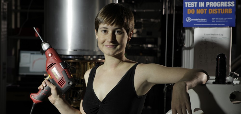


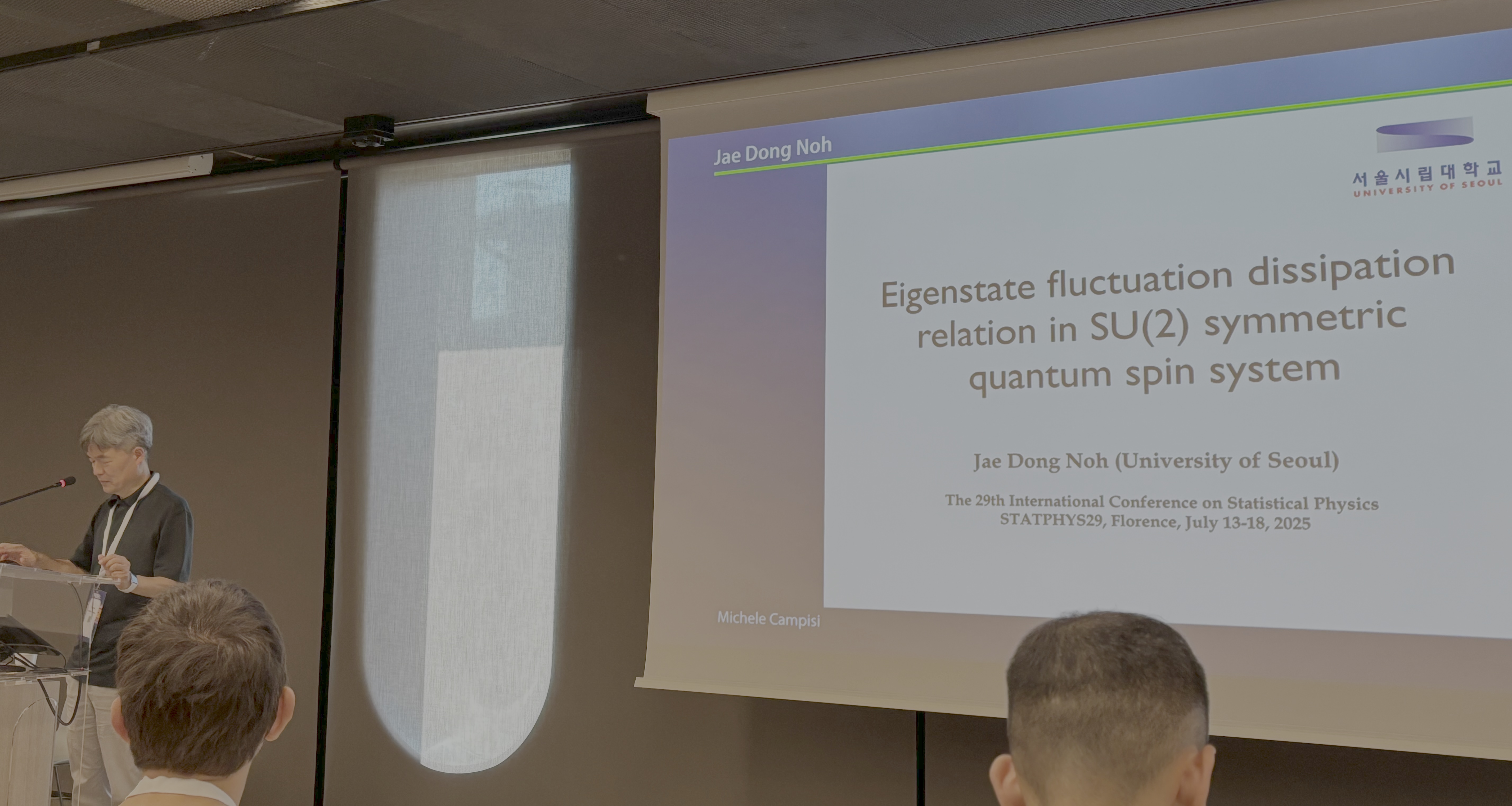


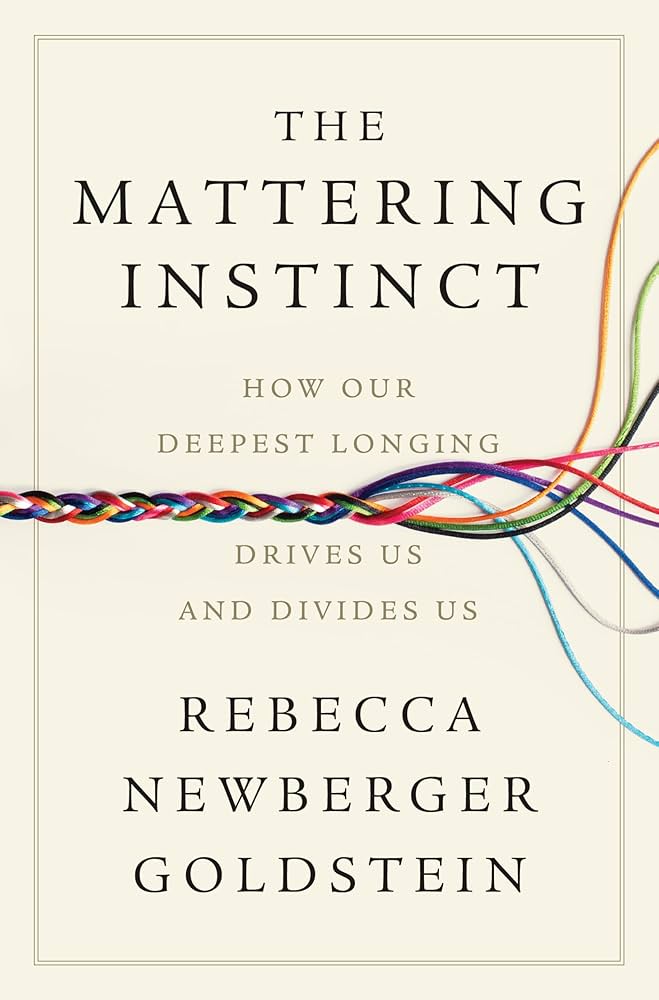
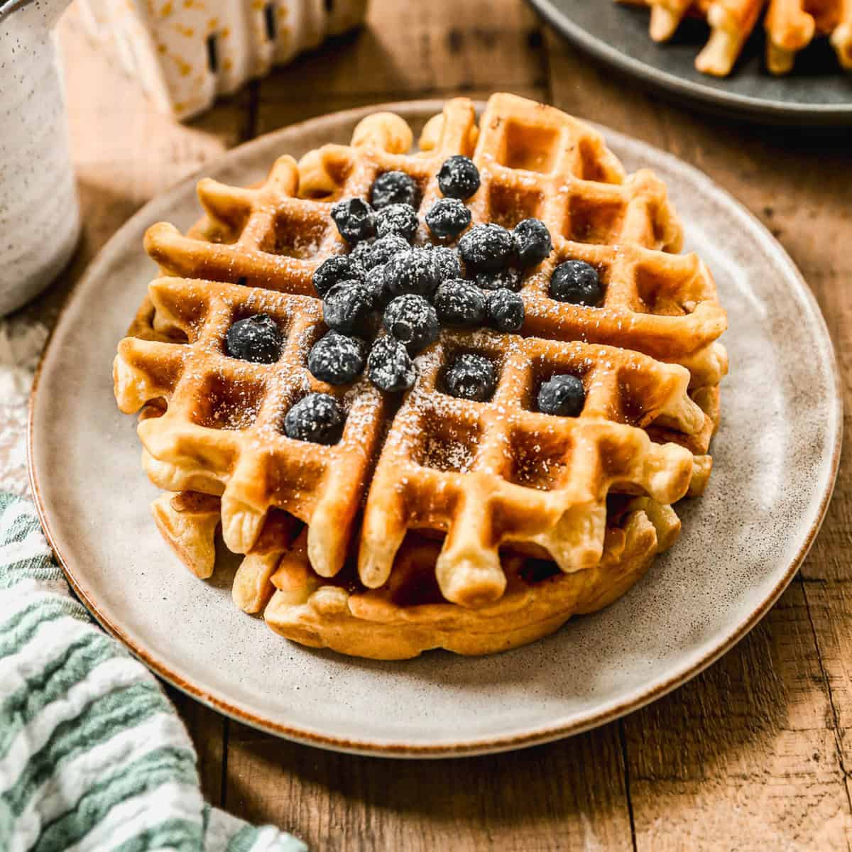

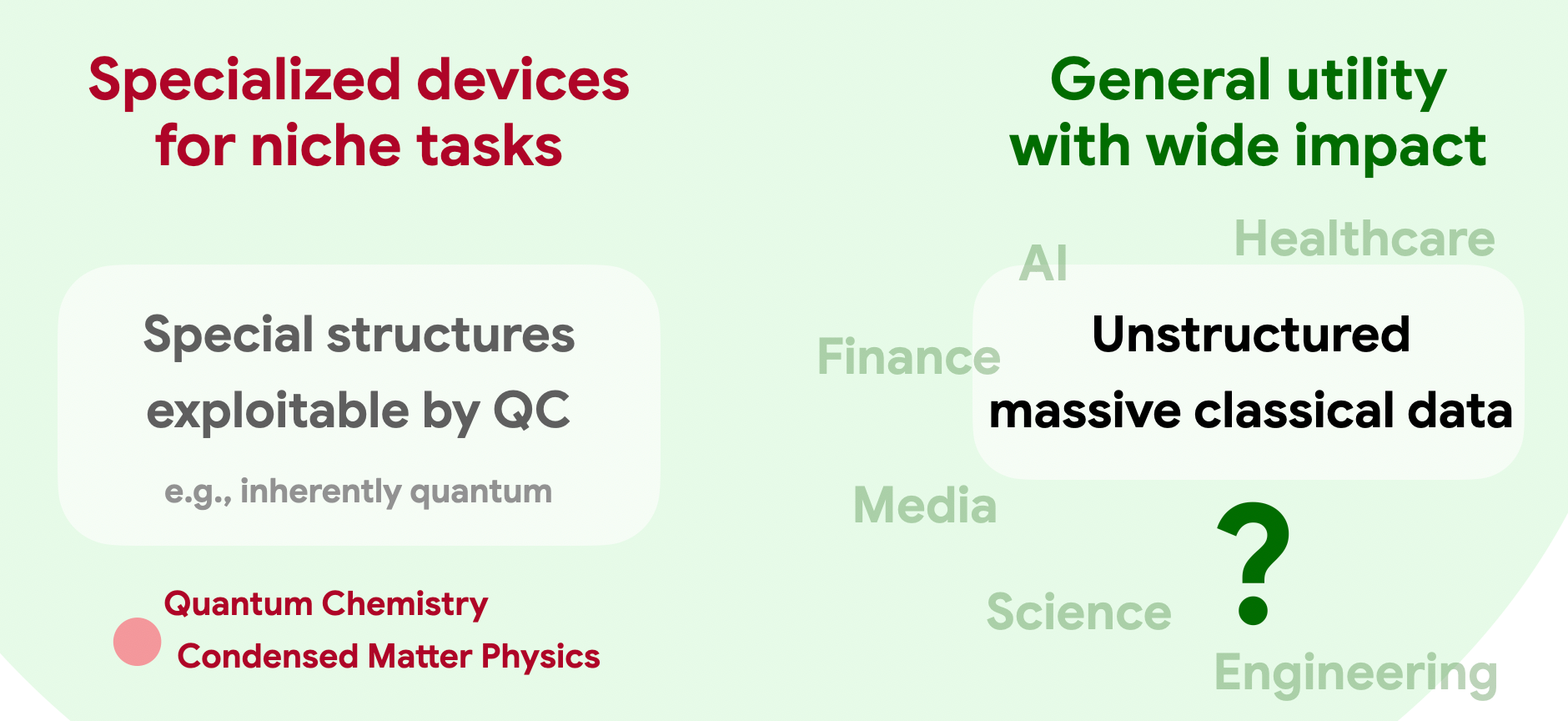
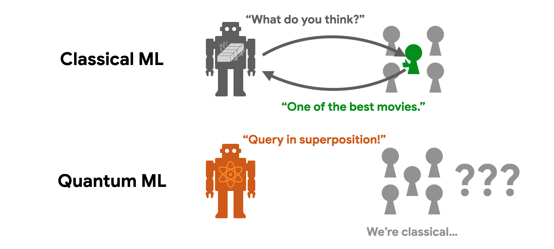
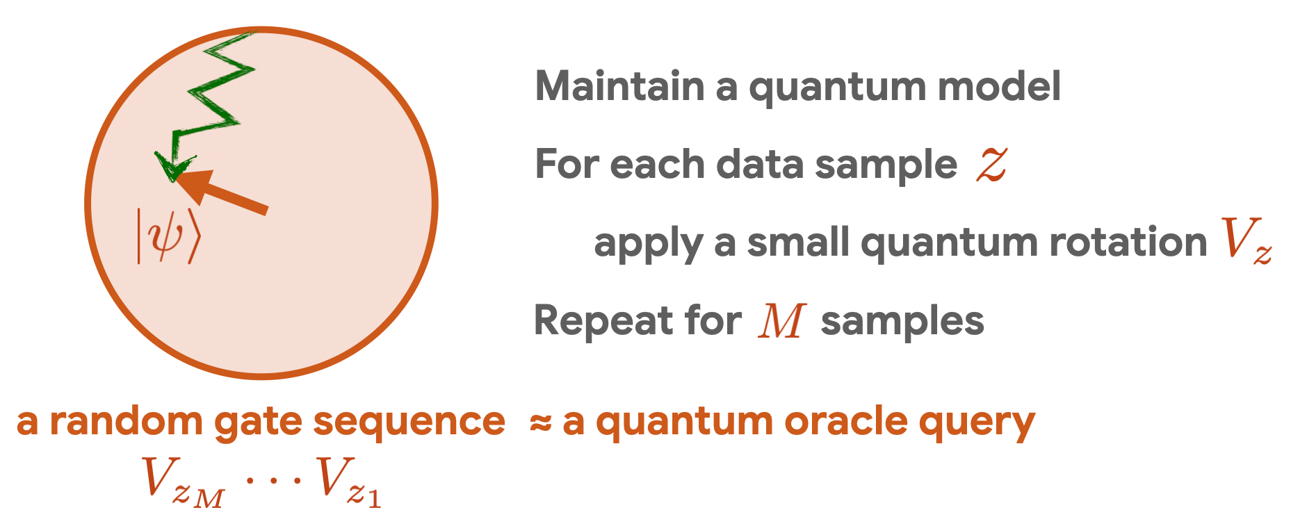
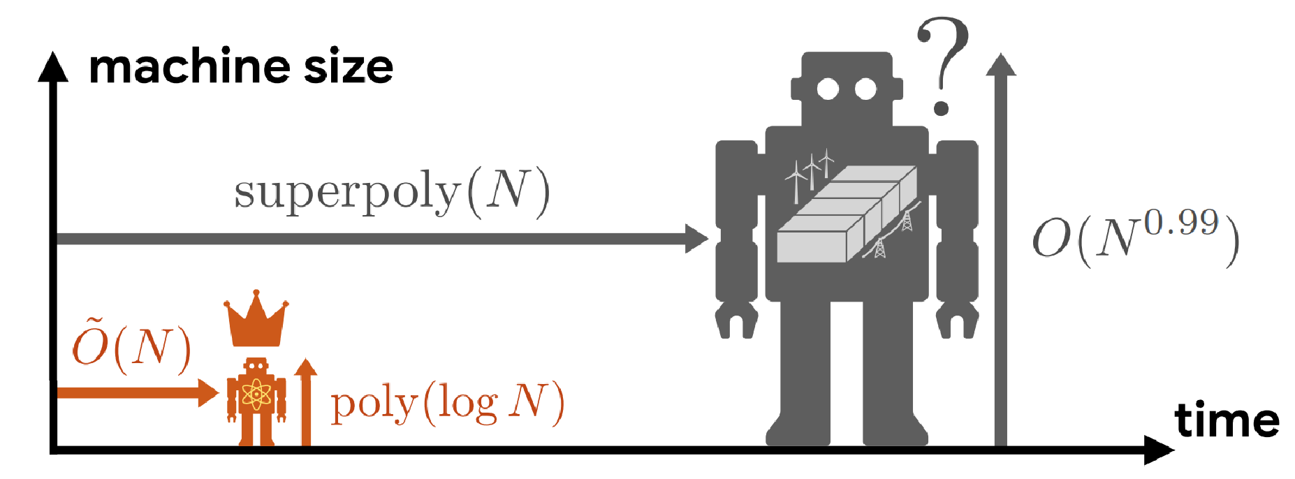
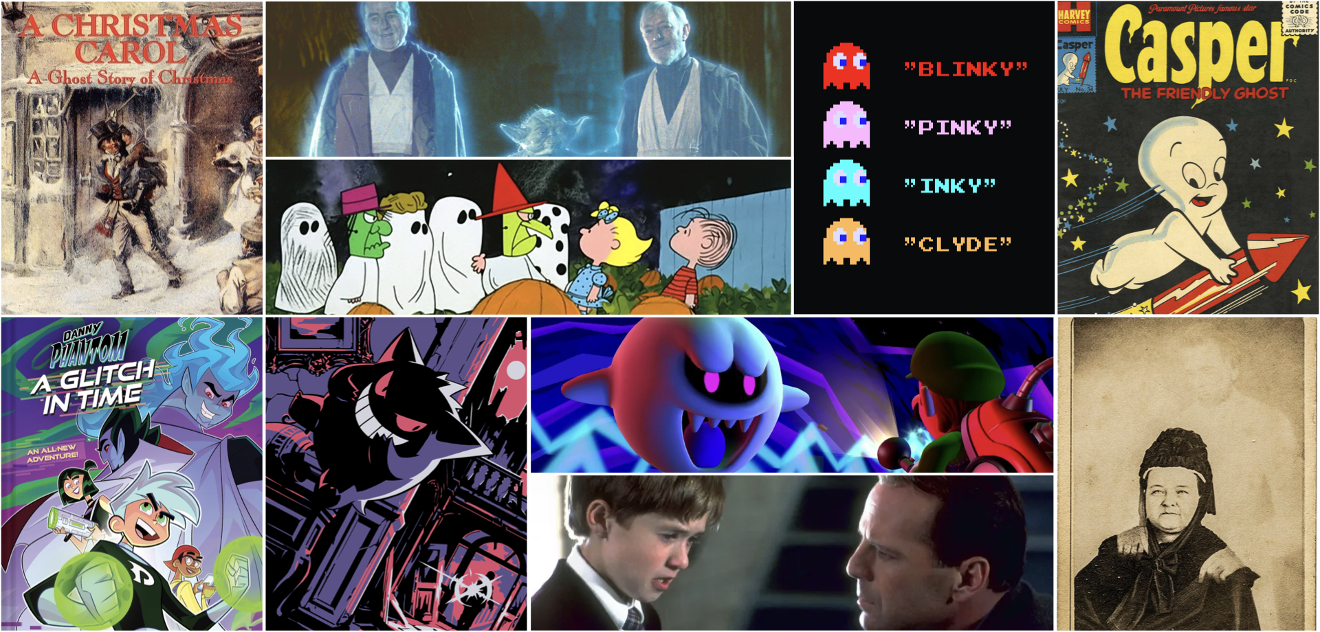
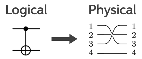
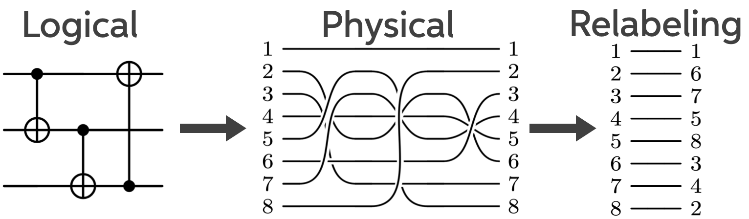
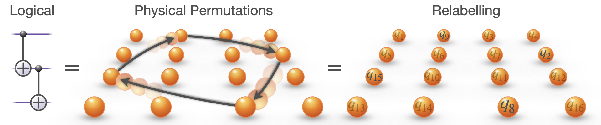
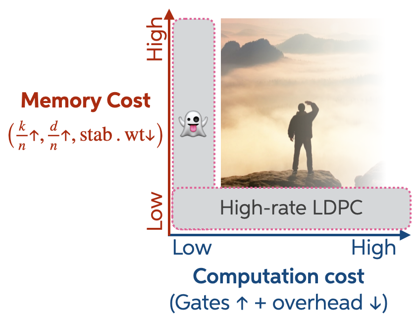
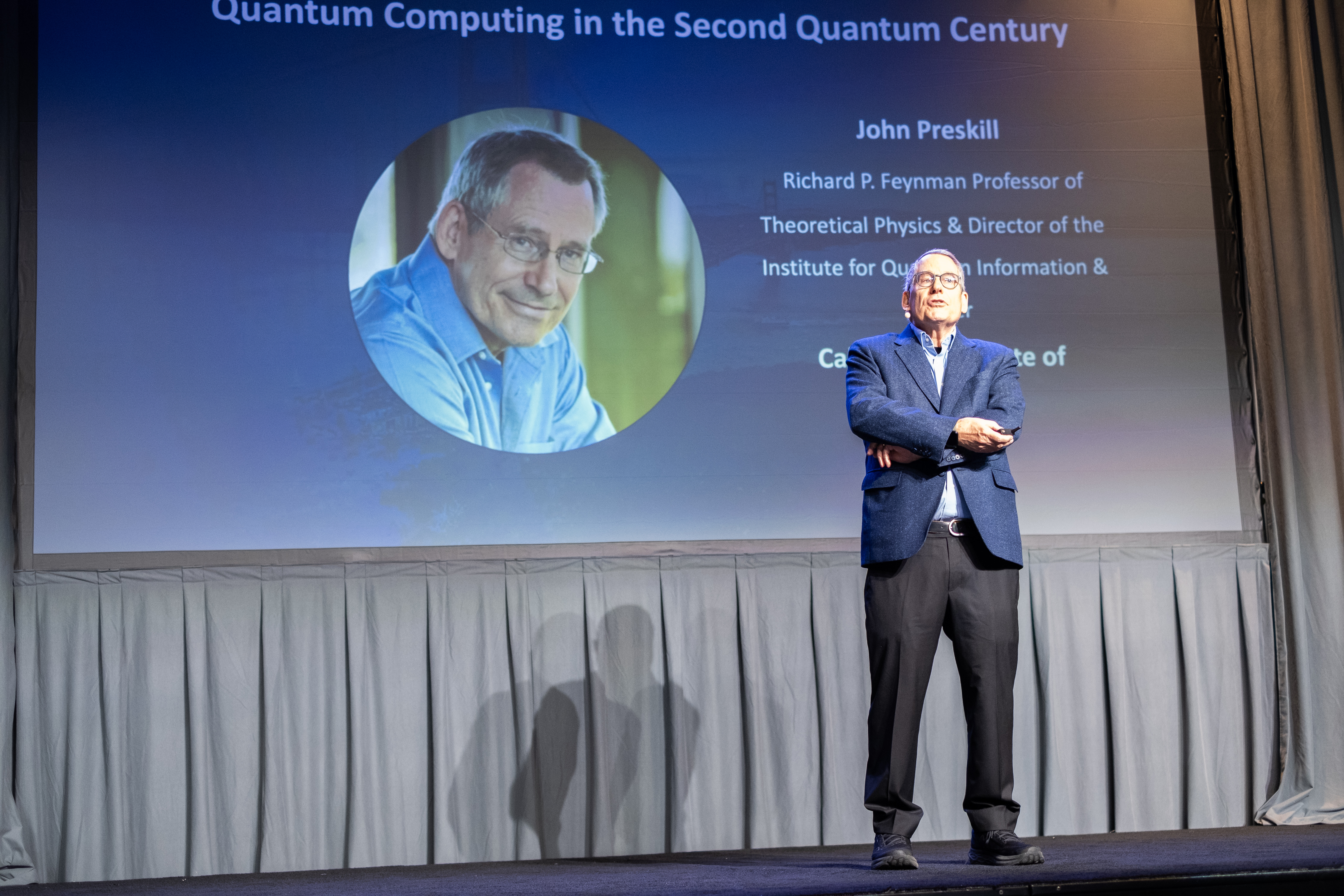


 . Farther up, the left-hand wire runs through a box. The box signifies that the corresponding qubit undergoes a transformation (for experts: a unitary evolution).


 of a particle, which may take two values,
  and
and  . Assumption 1 tells us that if Alice performs this measurement when the particle is in a superposition state, the joint system of Alice’s brain and the particle will end up in an entangled state. Now Alice’s mind-substrate is not in a pure state, so by Assumption 3 does not have a definite experience. This contradicts Assumption 2. Wigner’s proposed resolution to this paradox is that in fact Assumption 1 is incorrect, and that there is an influence of the mental on the physical, namely objective collapse or, as he puts it, that the “statistical element which, according to the orthodox theory, enters only if I make an observation enters equally if my friend does”.
 at time
  .” Then agent A can conclude that “I am certain that
  at time
  and
and  are certain about their respective judgments, since these states of knowledge change.
 , she knows that P” should be understood as claims about the state of the composite system composed of the part of Alice’s brain responsible for knowing P and the part responsible for recording outcomes of the measurement of q.


