Your inbox registers an email from the chair of a faculty-hiring committee. With trembling fingers, you click on the message. “We were very impressed…we’re delighted to offer…” Months of labor, soul-searching, strain, and anxiety give way to jubilation. You hug your partner/roommate/mom/dog; throw an impromptu dance party; and forward the email, prefaced with five exclamation points, to your mentor.1
As your heart rate returns to a level less likely to alarm a cardiologist, a new source of uncertainty puckers your brow. You’ve received an offer of a faculty position. What happens now? How should you proceed?
This article will address those questions. It follows my guide to faculty interviews, which follows my guide to writing research statements. Like the former guide, this one pertains most to theoretical physicists seeking assistant professorships at R1-level North American universities. Yet all the advice pertains to candidates outside this pool.
The institution will bring you (and, if relevant, your partner) over for a visit. Yes, you visited to interview; but you’re now visiting for another purpose. Assess whether you and your family could flourish if you accepted the offer. Which neighborhoods might you like to live in? Could you tolerate the commute to campus? Vide infra for more questions to keep in mind.
Politely notify the other hiring committees that interviewed you and that are still considering your application. You’ll do the other committees a kindness: their chances of hiring you have narrowed. If they wish to lure you, they’ll need to act quickly. The notice may bump you up in their priority lists. Did the first institution request that you decide about its offer by some deadline? If so, notify the other institutions.
Gather all the information you need. The department may offer to put you in touch with faculty members, deans, and more. Request more connections if necessary. Approach each conversation with a list of questions, and take notes. How will the tenure process unfold? How do early-career faculty members characterize their experiences with it? To what extent does the department shield early-career faculty from administrative duties (serving on committees)? How do the institutions’ policies address parental leave and elder care? If you have a child as an assistant professor, will your tenure clock pause for a year (will you be able to build your credentials for an extra year before applying for tenure)? In which neighborhoods should you search for a house?
List your priorities. Rank them. Measure each offer against each criterion. Here are example priorities that you might wish to include:
Salary
Startup package
Type of environment: Do you want to live in a city, in the suburbs, or in the country? Do you drive, or would you learn to drive?
Length of commute
Geographical location: Do you prefer to live near family?
Proximity, and means of transportation, to an airport: You might commute to and from that airport many times to participate in conferences, present seminars, etc. How much time and exhaustion would the experience cost?
Local school system: If you have or might have children, where would they learn?
Partner’s needs: Do you have a partner who would need to find a job near yours?
Proximity of faculty with whom you could collaborate
Courtesy positions in other departments: Suppose you’re a physicist who studies quantum computation. You might want to recruit students from the computer-science or math department occasionally. Could you? Would you need a courtesy position in the other department? A courtesy appointment offers you limited privileges at the cost of limited responsibilities: you probably won’t be able to vote in the other department’s faculty meetings. On the other hand, you probably won’t need to spend time on those faculty meetings.
Academic quality of undergraduate/graduate population
Presence of an institute/center dedicated to your specialization
Lab space: location, size, quality, renovations available, how soon and quickly the university would undertake those renovations
Help with finding housing: Some universities have apartments that new faculty can rent for a year or two. Other universities offer real-estate-agent services or help faculty obtain mortgages (*cough* San Francisco Bay area *cough*).
Administrative assistance for you and your research group
Protection from onerous service to the department until you reach tenure
Teaching relief granted en route to tenure: At some universities, a new faculty member can avoid teaching their usual course load during one or two semesters. Such relief frees you to buff up your research program while pursuing tenure.
Deferral: Deferring an offer, you postpone the time at which you take up the new mantle. When I accepted a permanent position, I was completing year two of a three-year postdoctoral fellowship. I wanted to complete the final year before assuming my new role: I was still finishing projects with the community to which I belonged, and I wanted to continue deepening my ties with that community. Also, I enjoyed undertaking research without the distraction of a primary investigator’s administrative responsibilities. Other people defer their start dates for other reasons. For example, a partner might need time to fulfill a contract where they live and work. In my experience, people tend to defer PI positions for approximately twelve months, give or take six months. Some institutions don’t offer deferrals, though.
Identify everything you’ll need in a startup package. A startup package helps cover your research program’s costs until you’ve won your first grants. Multiple organizations within a university might contribute to a startup package—for example, a department and an institute that cuts across departments. The hiring committee might propose a startup package to you, or the committee might ask you what you need. Either way, you can (and should) negotiate the package.
View the negotiation in terms of the question “What do I need to succeed?” List every item, and estimate its cost. Don’t skimp on rigor: estimate prices to the single-dollar level of precision. Such precision helps demonstrate the thoroughness of the research behind your list—helps demonstrate that you need every dollar you seek.
Request more funding than you believe you’ll need, because you will need more than you believe. Build the breathing room into your estimates. For example, assume that your academic visitors will fly from across the country or across the world. Assume that you’ll fly such distances to present talks. Estimating how much you’ll pay a student or postdoc throughout the next few years? Don’t forget that the university might raise salaries and benefits under a cost-of-living adjustment (COLA) every year. COLAs fluctuate across years, so assume you’ll face steep ones.
Here are examples of items that a startup package can include:
Summer salary: Your institution won’t pay your salary during the summer; you’ll need to fund yourself through grants. A startup package can cover the initial summers.
Lab equipment
Computers and tablets for you and your group members: Don’t forget protective cases, AppleCare or a non-Apple equivalent, implements for writing on tablets, external mice, and external monitors. Check whether your department or institute has spare mice or monitors that you can requisition.
Other computational resources: Does the department have a computational cluster that you intend to use? Do you need to access a national lab’s supercomputer or a quantum computer available on the cloud? How much will you pay per unit time and memory?
Postdoc costs: These costs include a salary, benefits, and the cost of moving to your institution. The salary will increase from year to year if the institution implements a COLA. The benefits include healthcare, dental care, and the like. Administrators might call benefits “fringe,” as I discovered after considerable confusion.
Graduate-student costs: These costs include a research assistantship, benefits, and possibly tuition. The salary might increase as a student progresses through the stages of their PhD, particularly once they achieve candidacy. Their need for tuition might change, too. Check whether domestic students cost more than international students, and budget for international students.
Undergraduate researchers: Do you plan to employ an undergraduate during the summer? Throughout the academic year?2
Travel for yourself: Budget several trips per year for yourself. You’ll need to spread the word about your research and to grow your network en route to tenure.
Travel for your postdocs and students: A mentor shared that she covers one conference per year per group member. You might want to budget also for a seminar or two per group member per year.
Visitors: Visitors can boost your research program. Budget for week-long visits if your institution can accommodate them.
Negotiate. Even if your dream school has offered you your dream job. Even if you receive only one offer. You might still garner resources that can help your research program and family to thrive. Don’t feel shy, sheepish, or ashamed to negotiate. If you remain polite and considerate, you won’t offend anyone. Besides, the hiring committee, department chair, and dean expect you to negotiate. The department chair might even hope that you do so; vide infra.
When I was a PhD student, Caltech offered a workshop about negotiation to women grad students. The workshop helped participants build skills, knowledge, and self-assurance that would benefit us when we negotiated contracts. I recommend attending a workshop, taking a course, reading a book, or watching videos about negotiation. Contact your institution’s professional-development office about opportunities and suggestions. If you’re reading this blog post before applying for jobs—any jobs—start now.
What can you negotiate for? Many of the items on your list of priorities. Certain institutions might lack the freedom to negotiate certain items, though. For example, a union might determine salaries. Don’t let such a discovery discourage you; explore the options thoroughly.
View the department chair as an ally. The department chair negotiates on your behalf with administrators higher up in the university hierarchy, such as deans. The chair aims to garner as many resources as possible for you—and, by extension, for their department. Explain to the department chair (or to the committee chair who might explain to the department chair) what you need and why you need it, to help strengthen their argument.
As soon as you know you’ll decline an offer, decline it politely. Your notification will free the committee to attract another candidate. Imagine you’re Candidate #2 on the priority list. Wouldn’t you want the current offer recipient to decline their offer as soon as their conscience allows? Now, imagine you’re the hiring-committee chair. You’re worried that Candidate #1 will decline—and, by the time they decline, other institutions will have snapped up the other top candidates. As Candidate #1, demonstrate toward the committee chair and toward Candidate #2 the consideration that you’d value if in their shoes.
Savor the moment. You’ve just survived the faculty-application process, one of the most stressful periods of your life. The faculty life is no walk in the park, either. Nor will you necessarily sleep soundly between the receipt of your first offer and your signing of a contract. The prospect of more offers could leave you in limbo. If you receive multiple offers, choosing between them—choosing the course of your and your family’s life—may stress you as much as applying did. So remember to feel grateful for the source of your anxiety. Give yourself credit for your accomplishment.
Congratulations!
1Please do! They’ll want to celebrate with you.
2I recommend targeting undergrads who’ll work with you for more than a summer. Training an undergrad takes nearly a summer; you and the student will benefit from having time to take advantage of that training.
We are now at an exciting point in our process of developing quantum computers and understanding their computational power: It has been demonstrated that quantum computers can outperform classical ones (if you buy my argument from Parts 1 and 2 of this mini series). And it has been demonstrated that quantum fault-tolerance is possible for at least a few logical qubits. Together, these form the elementary building blocks of useful quantum computing.
And yet: the devices we have seen so far are still nowhere near being useful for any advantageous application in, say, condensed-matter physics or quantum chemistry, which is where the promise of quantum computers lies.
So what is next in quantum advantage?
This is what this third and last part of my mini-series on the question “Has quantum advantage been achieved?” is about.
The 100 logical qubits regime I want to have in mind the regime in which we have 100 well-functioning logical qubits, so 100 qubits on which we can run maybe 100 000 gates.
Building devices operating in this regime will require thousand(s) of physical qubits and is therefore well beyond the proof-of-principle quantum advantage and fault-tolerance experiments that have been done. At the same time, it is (so far) still one or more orders of magnitude away from any of the first applications such as simulating, say, the Fermi-Hubbard model or breaking cryptography. In other words, it is a qualitatively different regime from the early fault-tolerant computations we can do now. And yet, there is not a clear picture for what we can and should do with such devices.
The next milestone: classically verifiable quantum advantage
In this post, I want to argue that a key milestone we should aim for in the 100 logical qubit regime is classically verifiable quantum advantage. Achieving this will not only require the jump in quantum device capabilities but also finding advantage schemes that allow for classical verification using these limited resources.
Why is it an interesting and feasible goal and what is it anyway?
To my mind, the biggest weakness of the RCS experiments is the way they are verified. I discussed this extensively in the last posts—verification uses XEB which can be classically spoofed, and only actually measured in the simulatable regime. Really, in a quantum advantage experiment I would want there to be an efficient procedure that will without any reasonable doubt convince us that a computation must have been performed by a quantum computer when we run it. In what I think of as classically verifiable quantum advantage, a (classical) verifier would come up with challenge circuits which they would then send to a quantum server. These would be designed in such a way that once the server returns classical samples from those circuits, the verifier can convince herself that the server must have run a quantum computation.
The theoretical computer scientist’s cartoon of verifying a quantum computer.
This is the jump from a physics-type experiment (the sense in which advantage has been achieved) to a secure protocol that can be used in settings where I do not want to trust the server and the data it provides me with. Such security may also allow a first application of quantum computers: to generate random numbers whose genuine randomness can be certified—a task that is impossible classically.
Here is the problem: On the one hand, we do know of schemes that allow us to classically verify that a computer is quantum and generate random numbers, so called cryptographic proofs of quantumness (PoQ). A proof of quantumness is a highly reliable scheme in that its security relies on well-established cryptography. Their big drawback is that they require a large number of qubits and operations, comparable to the resources required for factoring. On the other hand, the computations we can run in the advantage regime—basically, random circuits—are very resource-efficient but not verifiable.
The 100-logical-qubit regime lies right in the middle, and it seems more than plausible that classically verifiable advantage is possible in this regime. The theory challenge ahead of us is to find it: a quantum advantage scheme that is very resource-efficient like RCS and also classically verifiable like proofs of quantumness.
To achieve verifiable advantage in the 100-logical-qubit regime we need to close the gap between random circuit sampling and proofs of quantumness.
With this in mind, let me spell out some concrete goals that we can achieve using 100 logical qubits on the road to classically verifiable quantum advantage.
1. Demonstrate fault-tolerant quantum advantage
Before we talk about verifiable advantage, the first experiment I would like to see is one that combines the two big achievements of the past years, and shows that quantum advantage and fault-tolerance can be achieved simultaneously. Such an experiment would be similar in type to the RCS experiments, but run on encoded qubits with gate sets that match that encoding. During the computation, noise would be suppressed by correcting for errors using the code. In doing so, we could reach the near-perfect regime of RCS as opposed to the finite-fidelity regime that current RCS experiments operate in (as I discussed in detail in Part 2).
Random circuits with a quantum advantage that are particularly easy to implement fault-tolerantly are so-called IQP circuits. In those circuits, the gates are controlled-NOT gates and diagonal gates, so rotations , which just add a phase to a basis state as . The only “quantumness” comes from the fact that each input qubit is in the superposition state , and that all qubits are measured in the basis. This is an example of an example of an IQP circuit:
An IQP circuit starts from the all- state by applying a Hadamard transform, followed by IQP gates (in this case , some CNOT gates, , some CNOT gates, ) and ends in a measurement in the Hadamard basis.
As it so happens, IQP circuits are already really well understood since one of the first proposals for quantum advantage was based on IQP circuits (VerIQP1), and for a lot of the results in random circuits, we have precursors for IQP circuits, in particular, their ideal and noisy complexity (SimIQP). This is because their near-classical structure makes them relatively easy to study. Most importantly, their outcome probabilities are simple (but exponentially large) sums over phases that can just be read off from which gates are applied in the circuit and we can use well-established classical techniques like Boolean analysis and coding theory to understand those.
IQP gates are natural for fault-tolerance because there are codes in which all the operations involved can be implemented transversally. This means that they only require parallel physical single- or two-qubit gates to implement a logical gate rather than complicated fault-tolerant protocols which are required for universal circuits. This is in stark contrast to universal circuit which require resource-intensive fault-tolerant protocols. Running computations with IQP circuits would also be a step towards running real computations in that they can involve structured components such as cascades of CNOT gates and the like. These show up all over fault-tolerant constructions of algorithmic primitives such as arithmetic or phase estimation circuits.
Our concrete proposal for an IQP-based fault-tolerant quantum advantage experiment in reconfigurable-atom arrays is based on interleaving diagonal gates and CNOT gates to achieve super-fast scrambling (ftIQP1). A medium-size version of this protocol was implemented by the Harvard group (LogicalExp) but with only a bit more effort, it could be performed in the advantage regime.
In those proposals, verification will still suffer from the same problems of standard RCS experiments, so what’s up next is to fix that!
2. Closing the verification loophole
I said that a key milestone for the 100-logical-qubit regime is to find schemes that lie in between RCS and proofs of quantumness in terms of their resource requirements but at the same time allow for more efficient and more convincing verification than RCS. Naturally, there are two ways to approach this space—we can make quantum advantage schemes more verifiable, and we can make proofs of quantumness more resource-efficient.
First, let’s focus on the former approach and set a more moderate goal than full-on classical verification of data from an untrusted server. Are there variants of RCS that allow us to efficiently verify that finite-fidelity RCS has been achieved if we trust the experimenter and the data they hand us?
2.1 Efficient quantum verification using random circuits with symmetries
Indeed, there are! I like to think of the schemes that achieve this as random circuits with symmetries. A symmetry is an operator such that the outcome state of the computation (or some intermediate state) is invariant under the symmetry, so . The idea is then to find circuits that exhibit a quantum advantage and at the same time have symmetries that can be easily measured, say, using only single-qubit measurements or a single gate layer. Then, we can use these measurements to check whether or not the pre-measurement state respects the symmetries. This is a test for whether the quantum computer prepared the correct state, because errors or deviations from the true state would violate the symmetry (unless they were adversarially engineered).
In random circuits with symmetries, we can thus use small, well-characterized measurements whose outcomes we trust to probe whether a large quantum circuit has been run correctly. This is possible in a scenario I call the trusted experimenter scenario.
The trusted experimenter scenario In this scenario, we receive data from an actual experiment in which we trust that certain measurements were actually and correctly performed.
I think of random circuits with symmetries as introducing measurements in the circuit that check for errors.
Here are some examples of random circuits with symmetries, which allow for efficient verification of quantum advantage in the trusted experimenter scenario.
Graph states. My first example are locally rotated graph states (GStates). These are states that are prepared by CZ gates acting according to the edges of a graph on an initial all- state, and a layer of single-qubit -rotations is performed before a measurement in the basis. (Yes, this is also an IQP circuit.) The symmetries of this circuit are locally rotated Pauli operators, and can therefore be measured using only single-qubit rotations and measurements. What is more, these symmetries fully determine the graph state. Determining the fidelity then just amounts to averaging the expectation values of the symmetries, which is so efficient you can even do it in your head. In this example, we need measuring the outcome state to obtain hard-to-reproduce samples and measuring the symmetries are done in two different (single-qubit) bases.
With 100 logical qubits, samples from classically intractable graph states on several 100 qubits could be easily generated.
Bell sampling. The drawback of this approach is that we need to make two different measurements for verification and sampling. But it would be much more neat if we could just verify the correctness of a set of classically hard samples by only using those samples. For an example where this is possible, consider two copies of the output state of a random circuit, so . This state is invariant under a swap of the two copies, and in fact the expectation value of the SWAP operator in a noisy state preparation of determines the purity of the state, so . It turns out that measuring all pairs of qubits in the state in the pairwise basis of the four Bell states , where is one of the four Pauli matrices , this is hard to simulate classically (BellSamp). You may also observe that the SWAP operator is diagonal in the Bell basis, so its expectation value can be extracted from the Bell-basis measurements—our hard to simulate samples. To do this, we just average sign assignments to the samples according to their parity.
If the circuit is random, then under the same assumptions as those used in XEB for random circuits, the purity is a good estimator of the fidelity, so . So here is an example, where efficient verification is possible directly from hard-to-simulate classical samples under the same assumptions as those used to argue that XEB equals fidelity.
With 100 logical qubits, we can achieve quantum advantage which is at least as hard as the current RCS experiments that can also be efficiently (physics-)verified from the classical data.
Fault-tolerant circuits. Finally, suppose that we run a fault-tolerant quantum advantage experiment. Then, there is a natural set of symmetries of the state at any point in the circuit, namely, the stabilizers of the code we use. In a fault-tolerant experiment we repeatedly measure those stabilizers mid-circuit, so why not use that data to assess the quality of the logical state? Indeed, it turns out that the logical fidelity can be estimated efficiently from stabilizer expectation values even in situations in which the logical circuit has a quantum advantage (SyndFid).
With 100 logical qubits, we could therefore just run fault-tolerant IQP circuits in the advantage regime (ftIQP1) and the syndrome data would allow us to estimate the logical fidelity.
In all of these examples of random circuits with symmetries, coming up with classical samples that pass the verification tests is very easy, so the trusted-experimenter scenario is crucial for this to work. (Note, however, that it may be possible to add tests to Bell sampling that make spoofing difficult.) At the same time, these proposals are very resource-efficient in that they only increase the cost of a pure random-circuit experiment by a relatively small amount. What is more, the required circuits have more structure than random circuits in that they typically require gates that are natural in fault-tolerant implementations of quantum algorithms.
Performing random circuit sampling with symmetries is therefore a natural next step en-route to both classically verifiable advantage that closes the no-efficient verification loophole, and towards implementing actual algorithms.
What if we do not want to afford that level of trust in the person who runs the quantum circuit, however?
2.2 Classical verification using random circuits with planted secrets
If we do not trust the experimenter, we are in the untrusted quantum server scenario.
The untrusted quantum server scenario In this scenario, we delegate a quantum computation to an untrusted (presumably remote) quantum server—think of using a Google or Amazon cloud server to run your computation. We can communicate with this server using classical information.
In the untrusted server scenario, we can hope to use ideas from proofs of quantumness such as the use of classical cryptography to design families of quantum circuits in which some secret structure is planted. This secret structure should give the verifier a way to check whether a set of samples passes a certain verification test. At the same time it should not be detectable, or at least not be identifiable from the circuit description alone.
The simplest example of such secret structure could be a large peak in an otherwise flat output distribution of a random-looking quantum circuit. To do this, the verifier would pick a (random) string and design a circuit such that the probability of seeing in samples, is large. If the peak is hidden well, finding it just from the circuit description would require searching through all of the outcome bit strings and even just determining one of the outcome probabilities is exponentially difficult. A classical spoofer trying to fake the samples from a quantum computer would then be caught immediately: the list of samples they hand the verifier will not even contain unless they are unbelievably lucky, since there are exponentially many possible choices of .
Unfortunately, planting such secrets seems to be very difficult using universal circuits, since the output distributions are so unstructured. This is why we have not yet found good candidates of circuits with peaks, but some tries have been made (Peaks,ECPeaks,HPeaks)
We do have a promising candidate, though—IQP circuits! The fact that the output distributions of IQP circuits are quite simple could very well help us design sampling schemes with hidden secrets. Indeed, the idea of hiding peaks has been pioneered by Shepherd and Bremner (VerIQP1) who found a way to design classically hard IQP circuits with a large hidden Fourier coefficient. The presence of this large Fourier coefficient can easily be checked from a few classical samples, and random IQP circuits do not have any large Fourier coefficients. Unfortunately, for that construction and a variation thereof (VerIQP2), it turned out that the large coefficient can be detected quite easily from the circuit description (ClassIQP1,ClassIQP2).
To this day, it remains an exciting open question whether secrets can be planted in (maybe IQP) circuit families in a way that allows for efficient classical verification. Even finding a scheme with some large gap between verification and simulation times would be exciting, because it would for the first time allow us to verify a quantum computing experiment in the advantage regime using only classical computation.
Towards applications: certifiable random number generation
Beyond verified quantum advantage, sampling schemes with hidden secrets may be usable to generate classically certifiable random numbers: You sample from the output distribution of a random circuit with a planted secret, and verify that the samples come from the correct distribution using the secret. If the distribution has sufficiently high entropy, truly random numbers can be extracted from them. The same can be done for RCS, except that some acrobatics are needed to get around the problem that verification is just as costly as simulation (CertRand, CertRandExp). Again, a large gap between verification and simulation times would probably permit such certified random number generation.
The goal here is firstly a theoretical one: Come up with a planted-secret RCS scheme that has a large verification-simulation gap. But then, of course, it is an experimental one: actually perform such an experiment to classically verify quantum advantage.
Should an IQP-based scheme of circuits with secrets exist, 100 logical qubits is the regime where it should give a relevant advantage.
Three milestones
Altogether, I proposed three milestones for the 100 logical qubit regime.
Perform fault-tolerant quantum advantage using random IQP circuits. This will allow an improvement of the fidelity towards performing near-perfect RCS and thus closes the scalability worries of noisy quantum advantage I discussed in my last post.
Perform RCS with symmetries. This will allow for efficient verification of quantum advantage in the trusted experimenter scenario and thus make a first step toward closing the verification loophole.
Find and perform RCS schemes with planted secrets. This will allow us to verify quantum advantage in the remote untrusted server scenario and presumably give a first useful application of quantum computers to generate classically certified random numbers.
All of these experiments are natural steps towards performing actually useful quantum algorithms in that they use more structured circuits than just random universal circuits and can be used to benchmark the performance of the quantum devices in an advantage regime. Moreover, all of them close some loophole of the previous quantum advantage demonstrations, just like follow-up experiments to the first Bell tests have closed the loopholes one by one.
I argued that IQP circuits will play an important role in achieving those milestones since they are a natural circuit family in fault-tolerant constructions and promising candidates for random circuit constructions with planted secrets. Developing a better understanding of the properties of the output distributions of IQP circuits will help us achieve the theory challenges ahead.
Experimentally, the 100 logical qubit regime is exactly the regime to shoot for with those circuits since while IQP circuits are somewhat easier to simulate than universal random circuits, 100 qubits is well in the classically intractable regime.
What I did not talk about
Let me close this mini-series by touching on a few things that I would have liked to discuss more.
First, there is the OTOC experiment by the Google team (OTOC) which has spawned quite a debate. This experiment claims to achieve quantum advantage for an arguably more natural task than sampling, namely, computing expectation values. Computing expectation values is at the heart of quantum-chemistry and condensed-matter applications of quantum computers. And it has the nice property that it is what the Google team called “quantum-verifiable” (and what I would call “hopefully-in-the-future-verifiable”) in the following sense: Suppose we perform an experiment to measure a classically hard expectation value on a noisy device now, and suppose this expectation value actually carries some signal, so it is significantly far away from zero. Once we have a trustworthy quantum computer in the future, we will be able to check that the outcome of this experiment was correct and hence quantum advantage was achieved. There is a lot of interesting science to discuss about the details of this experiment and maybe I will do so in a future post.
Finally, I want to mention an interesting theory challenge that relates to the noise-scaling arguments I discussed in detail in Part 2: The challenge is to understand whether quantum advantage can be achieved in the presence of a constant amount of local noise. What do we know about this? On the one hand, log-depth random circuits with constant local noise are easy to simulate classically (SimIQP,SimRCS), and we have good numerical evidence that random circuits at very low depths are easy to simulate classically even without noise (LowDSim). So is there a depth regime in between the very low depth and the log-depth regime in which quantum advantage persists under constant local noise? Is this maybe even true in a noise regime that does not permit fault-tolerance (see this interesting talk)? In the regime in which fault-tolerance is possible, it turns out that one can construct simple fault-tolerance schemes that do not require any quantum feedback, so there are distributions that are hard to simulate classically even in the presence of constant local noise.
So long, and thanks for all the fish!
I hope that in this mini-series I could convince you that quantum advantage has been achieved. There are some open loopholes but if you are happy with physics-level experimental evidence, then you should be convinced that the RCS experiments of the past years have demonstrated quantum advantage.
As the devices are getting better at a rapid pace, there is a clear goal that I hope will be achieved in the 100-logical-qubit regime: demonstrate fault-tolerant and verifiable advantage (for the experimentalists) and come up with the schemes to do that (for the theorists)! Those experiments would close the loopholes of the current RCS experiments. And they would work as a stepping stone towards actual algorithms in the advantage regime.
I want to end with a huge thanks to Spiros Michalakis, John Preskill and Frederik Hahn who have patiently read and helped me improve these posts!
References
Fault-tolerant quantum advantage
(ftIQP1) Hangleiter, D. et al. Fault-Tolerant Compiling of Classically Hard Instantaneous Quantum Polynomial Circuits on Hypercubes. PRX Quantum6, 020338 (2025).
(LogicalExp) Bluvstein, D. et al. Logical quantum processor based on reconfigurable atom arrays. Nature626, 58–65 (2024).
Random circuits with symmetries
(BellSamp) Hangleiter, D. & Gullans, M. J. Bell Sampling from Quantum Circuits. Phys. Rev. Lett.133, 020601 (2024).
(GStates) Ringbauer, M. et al. Verifiable measurement-based quantum random sampling with trapped ions. Nat Commun16, 1–9 (2025).
(SyndFid) Xiao, X., Hangleiter, D., Bluvstein, D., Lukin, M. D. & Gullans, M. J. In-situ benchmarking of fault-tolerant quantum circuits. I. Clifford circuits. arXiv:2601.21472 II. Circuits with a quantum advantage. (coming soon!)
Verification with planted secrets
(PoQ) Brakerski, Z., Christiano, P., Mahadev, U., Vazirani, U. & Vidick, T. A Cryptographic Test of Quantumness and Certifiable Randomness from a Single Quantum Device. in 2018 IEEE 59th Annual Symposium on Foundations of Computer Science (FOCS) 320–331 (2018).
(VerIQP1) Shepherd, D. & Bremner, M. J. Temporally unstructured quantum computation. Proceedings of the Royal Society of London A: Mathematical, Physical and Engineering Sciences465, 1413–1439 (2009).
(VerIQP2) Bremner, M. J., Cheng, B. & Ji, Z. Instantaneous Quantum Polynomial-Time Sampling and Verifiable Quantum Advantage: Stabilizer Scheme and Classical Security. PRX Quantum6, 020315 (2025).
(ClassIQP1) Kahanamoku-Meyer, G. D. Forging quantum data: classically defeating an IQP-based quantum test. Quantum7, 1107 (2023).
(ClassIQP2) Gross, D. & Hangleiter, D. Secret-Extraction Attacks against Obfuscated Instantaneous Quantum Polynomial-Time Circuits. PRX Quantum6, 020314 (2025).
(Peaks) Aaronson, S. & Zhang, Y. On verifiable quantum advantage with peaked circuit sampling. arXiv:2404.14493
(ECPeaks) Deshpande, A., Fefferman, B., Ghosh, S., Gullans, M. & Hangleiter, D. Peaked quantum advantage using error correction. arXiv:2510.05262
(HPeaks) Gharibyan, H. et al. Heuristic Quantum Advantage with Peaked Circuits. arXiv:2510.25838
Certifiable random numbers
(CertRand) Aaronson, S. & Hung, S.-H. Certified Randomness from Quantum Supremacy. in Proceedings of the 55th Annual ACM Symposium on Theory of Computing 933–944 (Association for Computing Machinery, New York, NY, USA, 2023).
(CertRandExp) Liu, M. et al. Certified randomness amplification by dynamically probing remote random quantum states. arXiv:2511.03686
OTOC
(OTOC) Abanin, D. A. et al. Observation of constructive interference at the edge of quantum ergodicity. Nature646, 825–830 (2025).
Noisy complexity
(SimIQP) Bremner, M. J., Montanaro, A. & Shepherd, D. J. Achieving quantum supremacy with sparse and noisy commuting quantum computations. Quantum1, 8 (2017).
(SimRCS) Aharonov, D., Gao, X., Landau, Z., Liu, Y. & Vazirani, U. A polynomial-time classical algorithm for noisy random circuit sampling. in Proceedings of the 55th Annual ACM Symposium on Theory of Computing 945–957 (2023).
(LowDSim) Napp, J. C., La Placa, R. L., Dalzell, A. M., Brandão, F. G. S. L. & Harrow, A. W. Efficient Classical Simulation of Random Shallow 2D Quantum Circuits. Phys. Rev. X12, 021021 (2022).
My top 10 ghosts (solo acts and ensembles). If Bruce Willis being a ghost in The Sixth Sense is a spoiler, that’s on you — the movie has been out for 26 years.
Einstein and I have both been spooked by entanglement. Einstein’s experience was more profound: in a 1947 letter to Born, he famously dubbed it spukhafte Fernwirkung (or spooky action at a distance). Mine, more pedestrian. It came when I first learned the cost of entangling logical qubits on today’s hardware.
Logical entanglement is not easy
I recently listened to a talk where the speaker declared that “logical entanglement is easy,” and I have to disagree. You could argue that it looks easy when compared to logical small-angle gates, in much the same way I would look small standing next to Shaquille O’Neal. But that doesn’t mean 6’5” and 240 pounds is small.
To see why it’s not easy, it helps to look at how logical entangling gates are actually implemented. A logical qubit is not a single physical object. It’s an error-resistant qubit built out of several noisy, error-prone physical qubits. A quantum error-correcting (QEC) code with parameters uses physical qubits to encode logical qubits in a way that can detect up to physical errors and correct up to of them.
This redundancy is what makes fault-tolerant quantum computing possible. It’s also what makes logical operations expensive.
On platforms like neutral-atom arrays and trapped ions, the standard approach is a transversal CNOT: you apply two-qubit gates pairwise across the code blocks (qubit in block A interacts with qubit in block B). That requires physical two-qubit gates to entangle the logical qubits of one code block with the logical qubits of another.
To make this less abstract, here’s a QuEra animation showing a transversal CNOT implemented in a neutral-atom array. This animation is showing real experimental data, not a schematic idealization.
The idea is simple. The problem is that can be large, and physical two-qubit gates are among the noisiest operations available on today’s hardware.
Superconducting platforms take a different route. They tend to rely on lattice surgery; you entangle logical qubits by repeatedly measuring joint stabilizers along a boundary. That replaces two-qubit gates for stabilizer measurements over multiple rounds (typically scaling with the code distance). Unfortunately, physical measurements are the other noisiest primitive we have.
Then there are the modern high-rate qLDPC codes, which pack many logical qubits into a single code block. These are excellent quantum memories. But when it comes to computation, they face challenges. Logical entangling gates can require significant circuit depth, and often entire auxiliary code blocks are needed to mediate the interaction.
This isn’t a purely theoretical complaint. In recent state-of-the-art experiments by Google and by the Harvard–QuEra–MIT collaboration, logical entangling gates consumed nearly half of the total error budget.
So no, logical entanglement is not easy. But, how easy can we make it?
Phantom codes: Logical entanglement without physical operations
To answer how easy logical entanglement can really be, it helps to start with a slightly counterintuitive observation: logical entanglement can sometimes be generated purely by permuting physical qubits.
Let me show you how this works in the simplest possible setting, and then I’ll explain what’s really going on.
Consider a stabilizer code, which encodes 4 physical qubits into 2 logical ones that can detect 1 error, but can’t correct any. Below are its logical operators; the arrow indicates what happens when we physically swap qubits 1 and 3 (bars denote logical operators).
You can check that the logical operators transform exactly as shown, which is the action of a logical CNOT gate. For readers less familiar with stabilizer codes, click the arrow below for an explanation of what’s going on. Those familiar can carry on.
Click!
At the logical level, we identify gates by how they transform logical Pauli operators. This is the same idea used in ordinary quantum circuits: a gate is defined not just by what it does to states, but by how it reshuffles observables.
A CNOT gate has a very characteristic action. If qubit 1 is the control and qubit 2 is the target, then: an on the control spreads to the target, a on the target spreads back to the control, and the other Pauli operators remain unchanged.
That’s exactly what we see above.
To see why this generates entanglement, it helps to switch from operators to states. A canonical example of how to generate entanglement in quantum circuits is the following. First, you put one qubit into a superposition using a Hadamard. Starting from , this gives
At this point there is still no entanglement — just superposition.
The entanglement appears when you apply a CNOT. The CNOT correlates the two branches of the superposition, producing
which is a maximally-entangled Bell state. The Hadamard creates superposition; the CNOT turns that superposition into correlation.
The operator transformations above are simply the algebraic version of this story. Seeing
tells us that information on one logical qubit is now inseparable from the other.
In other words, in this code,
The figure below shows how this logical circuit maps onto a physical circuit. Each horizontal line represents a qubit. On the left is a logical CNOT gate: the filled dot marks the control qubit, and the ⊕ symbol marks the target qubit whose state is flipped if the control is in the state . On the right is the corresponding physical implementation, where the logical gate is realized by acting on multiple physical qubits.
At this point, all we’ve done is trade one physical operation for another. The real magic comes next. Physical permutations do not actually need to be implemented in hardware. Because they commute cleanly through arbitrary circuits, they can be pulled to the very end of a computation and absorbed into a relabelling of the final measurement outcomes. No operator spread. No increase in circuit depth.
This is not true for generic physical gates. It is a unique property of permutations.
To see how this works, consider a slightly larger example using an code. Here the logical operators are a bit more complicated:
Below is a three-logical-qubit circuit implemented using this code like the circuit drawn above, but now with an extra step. Suppose the circuit contains three logical CNOTs, each implemented via a physical permutation.
Instead of executing any of these permutations, we simply keep track of them classically and relabel the outputs at the end. From the hardware’s point of view, nothing happened.
If you prefer a more physical picture, imagine this implemented with atoms in an array. The atoms never move. No gates fire. The entanglement is there anyway.
This is the key point. Because no physical gates are applied, the logical entangling operation has zero overhead. And for the same reason, it has perfect fidelity. We’ve reached the minimum possible cost of a logical entangling gate. You can’t beat free.
To be clear, not all codes are amenable to logical entanglement through relabeling. This is a very special feature that exists in some codes.
Motivated by this observation, my collaborators and I defined a new class of QEC codes. I’ll state the definition first, and then unpack what it really means.
Phantom codes are stabilizer codes in which logical entangling gates between every ordered pair of logical qubits can be implemented solely via physical qubit permutations.
The phrase “every ordered pair” is a strong requirement. For three logical qubits, it means the code must support logical CNOTs between qubits , , , , , and . More generally, a code with logical qubits must support all possible directed CNOTs. This isn’t pedantry. Without access to every directed pair, you can’t freely build arbitrary entangling circuits — you’re stuck with a restricted gate set.
The phrase “solely via physical qubit permutations” is just as demanding. If all but one of those CNOTs could be implemented via permutations, but the last one required even a single physical gate — say, a one-qubit Clifford — the code would not be phantom. That condition is what buys you zero overhead and perfect fidelity. Permutations can be compiled away entirely; any additional physical operation cannot.
Together, these two requirements carve out a very special class of codes. All in-block logical entangling gates are free. Logical entangling gates between phantom code blocks are still available — they’re simply implemented transversally.
After settling on this definition, we went back through the literature to see whether any existing codes already satisfied it. We found two. The Carbon code and hypercube codes. The former enabled repeated rounds of quantum error-correction in trapped-ion experiments, while the latter underpinned recent neutral-atom experiments achieving logical-over-physical performance gains in quantum circuit sampling.
Both are genuine phantom codes. Both are also limited. With distance , they can detect errors but not correct them. With only logical qubits, there’s a limited class of CNOT circuits you can implement. Which begs the questions: Do other phantom codes exist? Can these codes have advantages that persist for scalable applications under realistic noise conditions? What structural constraints do they obey (parameters, other gates, etc.)?
Before getting to that, a brief note for the even more expert reader on four things phantom codes are not. Phantom codes are not a form of logical Pauli-frame tracking: the phantom property survives in the presence of non-Clifford gates. They are not strictly confined to a single code block: because they are CSS codes, multiple blocks can be stitched together using physical CNOTs in linear depth. They are not automorphism gates, which rely on single-qubit Cliffords and therefore do not achieve zero overhead or perfect fidelity. And they are not codes like SHYPS, Gross, or Tesseract codes, which allow only products of CNOTs via permutations rather than individually addressable ones. All of those codes are interesting. They’re just not phantom codes.
In a recent preprint, we set out to answer the three questions above. This post isn’t about walking through all of those results in detail, so here’s the short version. First, we find many more phantom codes — hundreds of thousands of additional examples, along with infinite families that allow both and to scale. We study their structural properties and identify which other logical gates they support beyond their characteristic phantom ones.
Second, we show that phantom codes can be practically useful for the right kinds of tasks — essentially, those that are heavy on entangling gates. In end-to-end noisy simulations, we find that phantom codes can outperform the surface code, achieving one–to–two orders of magnitude reductions in logical infidelity for resource state preparation (GHZ-state preparation) and many-body simulation, at comparable qubit overhead and with a modest preselection acceptance rate of about 24%.
If you’re interested in the details, you can read more in our preprint.
Larger space of codes to explore
This is probably a good moment to zoom out and ask the referee question: why does this matter?
I was recently updating my CV and realized I’ve now written my 40th referee report for APS. After a while, refereeing trains a reflex. No matter how clever the construction or how clean the proof, you keep coming back to the same question: what does this actually change?
So why do phantom codes matter? At least to me, there are two reasons: one about how we think about QEC code design, and one about what these codes can already do in practice.
The first reason is the one I’m most excited about. It has less to do with any particular code and more to do with how the field implicitly organizes the space of QEC codes. Most of that space is structured around familiar structural properties: encoding rate, distance, stabilizer weight, LDPC-ness. These form the axes that make a code a good memory. And they matter, a lot.
But computation lives on a different axis. Logical gates cost something, and that cost is sometimes treated as downstream—something to be optimized after a code is chosen, rather than something to design for directly. As a result, the cost of logical operations is usually inherited, not engineered.
One way to make this tension explicit is to think of code design as a multi-dimensional space with at least two axes. One axis is memory cost: how efficiently a code stores information. High rate, high distance, low-weight stabilizers, efficient decoding — all the usual virtues. The other axis is computational cost: how expensive it is to actually do things with the encoded qubits. Low computational cost means many logical gates can be implemented with little overhead. Low computational cost makes computation easy.
Why focus on extreme points in this space? Because extremes are informative. They tell you what is possible, what is impossible, and which tradeoffs are structural rather than accidental.
Phantom codes sit precisely at one such extreme: they minimize the cost of in-block logical entanglement. That zero-logical-cost extreme comes with tradeoffs. The phantom codes we find tend to have high stabilizer weights, and for families with scalable , the number of physical qubits grows exponentially. These are real costs, and they matter.
Still, the important lesson is that even at this extreme point, codes can outperform LDPC-based architectures on well-chosen tasks. That observation motivates an approach to QEC code design in which the logical gates of interest are placed at the centre of the design process, rather than treated as an afterthought. This is my first takeaway from this work.
Second is that phantom codes are naturally well suited to circuits that are heavy on logical entangling gates. Some interesting applications fall into this category, including fermionic simulation and correlated-phase preparation. Combined with recent algorithmic advances that reduce the overhead of digital fermionic simulation, these code-level ideas could potentially improve near-term experimental feasibility.
Back to being spooked
The space of QEC codes is massive. Perhaps two axes are not enough. Stabilizer weight might deserve its own. Perhaps different applications demand different projections of this space. I don’t yet know the best way to organize it.
The size of this space is a little spooky — and that’s part of what makes it exciting to explore, and to see what these corners of code space can teach us about fault-tolerant quantum computation.
Welcome back to: Has quantum advantage been achieved?
In Part 1 of this mini-series on quantum advantage demonstrations, I told you about the idea of random circuit sampling (RCS) and the experimental implementations thereof. In this post, Part 2 out of 3, I will discuss the arguments and evidence for why I am convinced that the experiments demonstrate a quantum advantage.
Recall from Part 1 that to assess an experimental quantum advantage claim we need to check three criteria:
Does the experiment correctly solve a computational task?
Does it achieve a scalable advantage over classical computation?
Does it achieve an in-practice advantage over the best classical attempt at solving the task?
What’s the issue?
When assessing these criteria for the RCS experiments there is an important problem: The early quantum computers we ran them on were very far from being reliable and the computation was significantly corrupted by noise. How should we interpret this noisy data? Or more concisely:
Is random circuit sampling still classically hard even when we allow for whatever amount of noise the actual experiments had?
Can we be convinced from the experimental data that this task has actually been solved?
I want to convince you today that we have developed a very good understanding of these questions that gives a solid underpinning to the advantage claim. Developing that understanding required a mix of methodologies from different areas of science, including theoretical computer science, algorithm design, and physics and has been an exciting journey over the past years.
The noisy sampling task
Let us start by answering the base question. What computational task did the experiments actually solve?
Recall that, in the ideal RCS scenario, we are given a random circuit on qubits and the task is to sample from the output distribution of the state obtained from applying the circuit to a simple reference state. The output probability distribution of this state is determined by the Born rule when I measure every qubit in a fixed choice of basis.
Now what does a noisy quantum computer do when I execute all the gates on it and apply them to its state? Well, it prepares a noisy version of the intended state and once I measure the qubits, I obtain samples from the output distribution of that noisy state.
We should not make the task dependent on the specifics of that state or the noise that determined it, but we can define a computational task based on this observation by fixing how accurate that noisy state preparation is. The natural way to do this is to use the fidelity
which is just the overlap between the ideal state and the noisy state. The fidelity is 1 if the noisy state is equal to the ideal state, and 0 if it is perfectly orthogonal to it.
Finite-fidelity random circuit sampling Given a typical random circuit , sample from the output distribution of any quantum state whose fidelity with the ideal output state is at least .
Note that finite-fidelity RCS does not demand success for every circuit, but only for typical circuits from the random circuit ensemble. This matches what the experiments do: they draw random circuits and need the device to perform well on the overwhelming majority of those draws. Accordingly, when the experiments quote a single number as “fidelity”, it is really the typical (or, more precisely, circuit-averaged) fidelity that I will just call .
The noisy experiments claim to have solved finite-fidelity RCS for values of around 0.1%. What is more, they consistently achieve this value even as the circuit sizes are increased in the later experiments. Both the actual value and the scaling will be important later.
What is the complexity of finite-fidelity RCS?
Quantum advantage of finite-fidelity RCS
Let’s start off by supposing that the quantum computation is (nearly) perfectly executed, so the required fidelity is quite large, say, 90%. In this scenario, we have very good evidence based on computational complexity theory that there is a scalable and in-practice quantum advantage for RCS. This evidence is very strong, comparable to the evidence we have for the hardness of factoring and simulating quantum systems. The intuition behind it is that quantum output probabilities are extremely hard to compute because of a mechanism behind quantum advantages: destructive interference. If you are interested in the subtleties and the open questions, take a look at our survey.
The question is now, how far down in fidelity this classical hardness persists? Intuitively, the smaller we make , the easier finite-fidelity RCS should become for a classical algorithm (and a quantum computer, too), since the freedom we have in deviating from the ideal state in our simulation becomes larger and larger. This increases the possibility of finding a state that turns out to be easy to simulate within the fidelity constraint.
Somewhat surprisingly, though, finite-fidelity RCS seems to remain hard even for very small values of . I am not aware of any efficient classical algorithm that achieves the finite-fidelity task for significantly away from the baseline trivial value of . This is the value a maximally mixed or randomly picked state achieves because a random state has no correlation with the ideal state (or any other state), and is exactly what you expect in that case (while 0 would correspond to perfect anti-correlation).
One can save some classical runtime compared to solving near-ideal RCS by exploiting a reduced fidelity, but the costs remain exponential. To classically solve finite-fidelity RCS, the best known approaches are reported in the papers that performed classical simulations of finite-fidelity RCS with the parameters of the first Google and USTC experiment (classSim1, classSim2). To achieve this, however, they needed to approximately simulate the ideal circuits at an immense cost. To the best of my knowledge, all but those first two experiments are far out of reach for these algorithms.
Getting the scaling right: weak noise and low depth
So what is the right value of at which we can hope for a scalable and in-practice advantage of RCS experiments?
When thinking about this question, it is helpful to keep a model of the circuit in mind that a noisy experiment runs. So, let us consider a noisy circuit on qubits with layers of gates and single-qubit noise of strength on every qubit in every layer. In this scenario, the typical fidelity with the ideal state will decay as .
Any reasonably testable value of the fidelity needs to scale as , since eventually we need to estimate the average fidelity from the experimental samples and this typically requires at least samples, so exponentially small fidelities are experimentally invisible. The polynomial fidelity is also much closer to the near-ideal scenario (90%) than the trivial scenario (). While we cannot formally pin this down, the intuition behind the complexity-theoretic evidence for the hardness of near-ideal RCS persists into the regime: to sample up to such high precision, we still need a reasonably accurate estimate of the ideal probabilities, and getting this is computationally extremely difficult. Scalable quantum advantage in this regime is therefore a pretty safe bet.
How do the parameters of the experiment and the RCS instances need to scale with the number of qubits to experimentally achieve the fidelity regime? The limit to consider is one in which the noise rate decreases with the number of qubits, while the circuit depth is only allowed to increase very slowly. It depends on the circuit architecture, i.e., the choice of circuit connectivity, and the gate set, through a constant as I will explain in more detail below.
Weak-noise and low-depth scaling (Weak noise) The local noise rate of the quantum device scales as . (Low depth) The circuit depth scales as .
This limit is such that we have a scaling of the fidelity as for some constant . It is also a natural scaling limit for noisy devices whose error rates gradually improve through better engineering. You might be worried about the fact that the depth needs to be quite low but it turns out that there is a solid quantum advantage even for -depth circuits.
The precise definition of the weak-noise regime is motivated by the following observation. It turns out to be crucial for assessing the noisy data from the experiment.
Fidelity versus XEB: a phase transition
Remember from Part 1 that the experiments measured a quantity called the cross-entropy benchmark (XEB)
The XEB averages the ideal probabilities corresponding to the sampled outcomes from experiments on random circuits . Thus, it correlates the experimental and ideal output distributions of those random circuits. You can think of it as a “classical version” of the fidelity: If the experimental distribution is correct, the XEB will essentially be 1. If it is uniformly random, the XEB is 0.
The experiments claimed that the XEB is a good proxy for the circuit-averaged fidelity given by , and so we need to understand when this is true. Fortunately, in the past few years, alongside with the improved experiments, we have developed a very good understanding of this question (WN, Spoof2, PT1, PT2).
It turns out that the quality of correspondence between XEB and average fidelity depends strongly on the noise in the experimental quantum state. In fact, there is a sharp phase transition: there is an architecture-dependent constant such that when the experimental local noise rate , then the XEB is a good and reliable proxy for the average fidelity for any system size and circuit depth . This is exactly the weak-noise regime. Above that threshold, in the strong noise regime, the XEB is an increasingly bad proxy for the fidelity (PT1, PT2).
Let me be more precise: In the weak-noise regime, when we consider the decay of the XEB as a function of circuit depth , the rate of decay is given by , i.e., the XEB decays as . Meanwhile, in the strong-noise regime the rate of decay is constant, giving an XEB decay as for a constant . At the same time, the fidelity decays as regardless of the noise regime. Hence, in the weak-noise regime, the XEB is a good proxy of the fidelity, while in the strong noise regime, there is an exponentially increasing gap between the XEB (which remains large) and the fidelity (which continues to decay exponentially). regardless of the noise regime.
This is what the following plot shows. We computed it from an exact mapping of the behavior of the XEB to the dynamics of a statistical-mechanics model that can be evaluated efficiently. Using this mapping, we can also compute the noise threshold for whichever random circuit family and architecture you are interested in.
From (PT2). The -axis label is the decay rate of the XEB , the number of qubits and is the local noise rate.
Where are the experiments?
We are now ready to take a look at the crux when assessing the noisy data: Can we trust the reported XEB values as an estimator of the fidelity? If so, do the experiments solve finite-fidelity RCS in the solidly hard regime where ?
In their more recent paper (PT1), the Google team explicitly verified that the experiment is well below the phase transition, and it turns out that the first experiment was just at the boundary. The USTC experiments had comparable noise rates, and the Quantinuum experiment much better ones. Since fidelity decays as , but the reported XEB values stayed consistently around 0.1% as was increased, the experimental error rate of the experiments improved even better than the scaling required for the weak-noise regime, namely, more like . Altogether, the experiments are therefore in the weak-noise regime both in terms of absolute numbers relative to and the required scaling.
Of course, to derive the transition, we made some assumptions about the noise such as that the noise is local, and that it does not depend much on the circuit itself. In the advantage experiments, these assumptions about the noise are characterized and tested. This is done through a variety of means at increasing levels of complexity, including detailed characterization of the noise in individual gates, gates run in parallel, and eventually in a larger circuit. The importance of understanding the noise shows in the fact that a significant portion of the supplementary materials of the advantage experiments is dedicated to getting this right. All of this contributes to the experimental justification for using the XEB as a proxy for the fidelity!
The data shows that the experiments solved finite-fidelity RCS for values of above the constant value of roughly 0.1% as the experiments grew. In the following plot, I compare the experimental fidelity values to the near-ideal scenario on the one hand, and the trivial value on the other hand. Viewed at this scale, the values of for which the experiment solved finite-fidelity RCS are indeed vastly closer to the near-ideal value than the trivial baseline, which should boost our confidence that reproducing samples at a similar fidelity is extremely challenging.
The phase transition matters!
You might be tempted to say: “Well, but is all this really so important? Can’t I just use XEB and forget all about fidelity?”
The phase transition shows why that would change the complexity of the problem: in the strong-noise regime, XEB can stay high even when fidelity is exponentially small. And indeed, this discrepancy can be exploited by so-called spoofers for the XEB. These are efficient classical algorithms which can be used to succeed at a quantum advantage test even though they clearly do not achieve the intended advantage. These spoofers (Spoof1, Spoof2) can achieve high XEB scores comparable to those of the experiments and scaling like in the circuit depth for some constant .
Their basic idea is to introduce strong, judiciously chosen noise at specific circuit locations that has the effect of breaking up the simulation task up into smaller, much easier components, but at the same time still gives a high XEB score. In doing so, they exploit the strong-noise regime in which the XEB is a really bad proxy for the fidelity. This allows them to sample from states with exponentially low fidelity while achieving a high XEB value.
The discovery of the phase transition and the associated spoofers highlights the importance of modeling when assessing—and even formulating—the advantage claim based on noisy data.
But we can’t compute the XEB!
You might also be worried that the experiments did not actually compute the XEB in the advantage regime because to estimate it they would have needed to compute ideal probabilities—a task that is hard by definition of the advantage regime. Instead, they used a bunch of different ways to extrapolate the true XEB from XEB proxies (proxy of a proxy of the fidelity). Is this is a valid way of getting an estimate of the true XEB?
It totally is! Different extrapolations—from easy-to-simulate to hard-to-simulate, from small system to large system etc—all gave consistent answers for the experimental XEB value of the supremacy circuits. Think of this as having several lines that cross in the same point. For that crossing to be a coincidence, something crazy, conspiratorial must happen exactly when you move to the supremacy circuits from different directions. That is why it is reasonable to trust the reported value of the XEB.
That’s exactly how experiments work!
All of this is to say that establishing that the experiments correctly solved finite-fidelity RCS and therefore show quantum advantage involved a lot of experimental characterization of the noise as well as theoretical work to understand the effects of noise on the quantity we care about—the fidelity between the experimental and ideal states.
In this respect (and maybe also in the scale of the discovery), the quantum advantage experiments are similar to the recent experiments reporting discovery of the Higgs boson and gravitational waves. While I do not claim to understand any of the details, what I do understand is that in both experiments, there is an unfathomable amount of data that could not be interpreted without preselection and post-processing of the data, theories, extrapolations and approximations that model the experiment and measurement apparatus. All of those enter the respective smoking-gun plots that show the discoveries.
If you believe in the validity of experimental physics methodology, you should therefore also believe in the type of evidence underlying experimental claim of the quantum advantage demonstrations: that they sampled from the output distribution of a quantum state with the reported fidelities.
Put succinctly: If you believe in the Higgs boson and gravitational waves, you should probably also believe in the experimental demonstration of quantum advantage.
What are the counter-arguments?
The theoretical computer scientist
“The weak-noise limit is not physical. The appropriate scaling limit is one in which the local noise rate of the device is constant while the system size grows, and in that case, there is a classical simulation algorithm for RCS (SimIQP, SimRCS).”
In theoretical computer science, scaling of time or the system size in the input size is considered very natural: We say an algorithm is efficient if its runtime and space usage only depend polynomially on the input size.
But all scaling arguments are hypothetical concepts, and we only care about the scaling at relevant sizes. In the end, every scaling limit is going to hit the wall of physical reality—be it the amount of energy or human lifetime that limits the time of an algorithm, or the physical resources that are required to build larger and larger computers. To keep the scaling limit going as we increase the size of our computations, we need innovation that makes the components smaller and less noisy.
At the scales relevant to RCS, the scaling of the noise is benign and even natural. Why? Well, currently, the actual noise in quantum computers is not governed by the fundamental limit, but by engineering challenges. Realizing this limit therefore amounts to engineering improvements in the system size and noise rate that are achieved over time. Sure, at some point that scaling limit is also going to hit a fundamental barrier below which the noise cannot be improved. But we are surely far away from that limit, yet. What is more, already now logical qubits are starting to work and achieve beyond-breakeven fidelities. So even if the engineering improvements should flatten out from here onward, QEC will keep the noise limit going and even accelerate it in the intermediate future.
The complexity maniac
“All the hard complexity-theoretic evidence for quantum advantage is in the near-ideal regime, but now you are claiming advantage for the low-fidelity version of that task.”
This is probably the strongest counter-argument in my opinion, and I gave my best response above. Let me just add that this is a question about computational complexity. In the end, all of complexity theory is based on belief. The only real evidence we have for the hardness of any task is the absence of an efficient algorithm, or the reduction to a paradigmatic, well-studied task for which there is no efficient algorithm.
I am not sure how much I would bet that you cannot find an efficient algorithm for finite-fidelity RCS in the regime of the experiments, but it is certainly a pizza.
The enthusiastic skeptic
“There is no verification test that just depends on the classical samples, is efficient and does not make any assumptions about the device. In particular, you cannot unconditionally verify fidelity just from the classical samples. Why should I believe the data?”
Yes, sure, the current advantage demonstrations are not device-independent. But the comparison you should have in mind are Bell tests. The first proper Bell tests of Aspect and others in the 80s were not free of loopholes. They still allowed for contrived explanations of the data that did not violate local realism. Still, I can hardly believe that anyone would argue that Bell inequalities were not violated already back then.
As the years passed, these remaining loopholes were closed. To be a skeptic of the data, people needed to come up with more and more adversarial scenarios that could explain the data. We are working on the same to happen with quantum advantage demonstrations: come up with better schemes and better tests that require less and less assumptions or knowledge about the specifics of the device.
The “this is unfair” argument
“When you chose the gates and architecture of the circuit dependent on your device, you tailored the task too much to the device and that is unfair. Not even the different RCS experiments solve exactly the same task.”
This is not really an argument against the achievement of quantum advantage but more against the particular choices of circuit ensembles in the experiments. Sure, the specific computations solved are still somewhat tailored to the hardware itself and in this sense the experiments are not hardware-independent yet, but they still solve fine computational tasks. Moving away from such hardware-tailored task specifications is another important next step and we are working on it.
In the third and last part of this mini series I will address next steps in quantum advantage that aim at closing some of the remaining loopholes. The most important—and theoretically interesting—one is to enable efficient verification of quantum advantage using less or even no specific knowledge about the device that was used, but just the measurement outcomes.
References
(survey) Hangleiter, D. & Eisert, J. Computational advantage of quantum random sampling. Rev. Mod. Phys.95, 035001 (2023).
(classSim1) Pan, F., Chen, K. & Zhang, P. Solving the sampling problem of the Sycamore quantum circuits. Phys. Rev. Lett.129, 090502 (2022).
(classSim2) Kalachev, G., Panteleev, P., Zhou, P. & Yung, M.-H. Classical Sampling of Random Quantum Circuits with Bounded Fidelity. arXiv.2112.15083 (2021).
(WN) Dalzell, A. M., Hunter-Jones, N. & Brandão, F. G. S. L. Random Quantum Circuits Transform Local Noise into Global White Noise. Commun. Math. Phys.405, 78 (2024).
(PT1)vMorvan, A. et al. Phase transitions in random circuit sampling. Nature634, 328–333 (2024).
(PT2) Ware, B. et al. A sharp phase transition in linear cross-entropy benchmarking. arXiv:2305.04954 (2023).
(Spoof1) Barak, B., Chou, C.-N. & Gao, X. Spoofing Linear Cross-Entropy Benchmarking in Shallow Quantum Circuits. in 12th Innovations in Theoretical Computer Science Conference (ITCS 2021) (ed. Lee, J. R.) vol. 185 30:1-30:20 (2021).
(Spoof2) Gao, X. et al. Limitations of Linear Cross-Entropy as a Measure for Quantum Advantage. PRX Quantum5, 010334 (2024).
(SimIQP) Bremner, M. J., Montanaro, A. & Shepherd, D. J. Achieving quantum supremacy with sparse and noisy commuting quantum computations. Quantum1, 8 (2017).
(SimRCS) Aharonov, D., Gao, X., Landau, Z., Liu, Y. & Vazirani, U. A polynomial-time classical algorithm for noisy random circuit sampling. in Proceedings of the 55th Annual ACM Symposium on Theory of Computing 945–957 (2023).
Recently, I gave a couple of perspective talks on quantum advantage, one at the annual retreat of the CIQC and one at a recent KITP programme. I started off by polling the audience on who believed quantum advantage had been achieved. Just this one, simple question.
The audience was mostly experimental and theoretical physicists with a few CS theory folks sprinkled in. I was sure that these audiences would be overwhelmingly convinced of the successful demonstration of quantum advantage. After all, more than half a decade has passed since the first experimental claim (G1) of “quantum supremacy” as the patron of this blog’s institute called the idea “to perform tasks with controlled quantum systems going beyond what can be achieved with ordinary digital computers” (Preskill, p. 2) back in 2012. Yes, this first experiment by the Google team may have been simulated in the meantime, but it was only the first in an impressive series of similar demonstrations that became bigger and better with every year that passed. Surely, so I thought, a significant part of my audiences would have been convinced of quantum advantage even before Google’s claim, when so-called quantum simulation experiments claimed to have performed computations that no classical computer could do (e.g. (qSim)).
I could not have been more wrong.
In both talks, less than half of the people in the audience thought that quantum advantage had been achieved.
In the discussions that ensued, I came to understand what folks criticized about the experiments that have been performed and even the concept of quantum advantage to begin with. But more on that later. Most of all, it seemed to me, the community had dismissed Google’s advantage claim because of the classical simulation shortly after. It hadn’t quite kept track of all the advances—theoretical and experimental—since then.
In a mini-series of three posts, I want to remedy this and convince you that the existing quantum computers can perform tasks that no classical computer can do. Let me caution, though, that the experiments I am going to talk about solve a (nearly) useless task. Nothing of what I say implies that you should (yet) be worried about your bank accounts.
I will start off by recapping what quantum advantage is and how it has been demonstrated in a set of experiments over the past few years.
Part 1: What is quantum advantage and what has been done?
To state the obvious: we are now fairly convinced that noiseless quantum computers would be able solve problems efficiently that no classical computer could solve. In fact, we have been convinced of that already since the mid-90ies when Lloyd and Shor discovered two basic quantum algorithms: simulating quantum systems and factoring large numbers. Both of these are tasks where we are as certain as we could be that no classical computer can solve them. So why talk about quantum advantage 20 and 30 years later?
The idea of a quantum advantage demonstration—be it on a completely useless task even—emerged as a milestone for the field in the 2010s. Achieving quantum advantage would finally demonstrate that quantum computing was not just a random idea of a bunch of academics who took quantum mechanics too seriously. It would show that quantum speedups are real: We can actually build quantum devices, control their states and the noise in them, and use them to solve tasks which not even the largest classical supercomputers could do—and these are very large.
What is quantum advantage?
But what exactly do we mean by “quantum advantage”. It is a vague concept, for sure. But some essential criteria that a demonstration should certainly satisfy are probably the following.
The quantum device needs to solve a pre-specified computational task. This means that there needs to be an input to the quantum computer. Given the input, the quantum computer must then be programmed to solve the task for the given input. This may sound trivial. But it is crucial because it delineates programmable computing devices from just experiments on any odd physical system.
There must be a scaling difference in the time it takes for a quantum computer to solve the task and the time it takes for a classical computer. As we make the problem or input size larger, the difference between the quantum and classical solution times should increase disproportionately, ideally exponentially.
And finally: the actual task solved by the quantum computer should not be solvable by any classical machine (at the time).
Achieving this last criterion using imperfect, noisy quantum devices is the challenge the idea of quantum supremacy set for the field. After all, running any of our favourite quantum algorithms in a classically hard regime on these devices is completely out of the question. They are too small and too noisy. So the field had to come up with the conceivably smallest and most noise-robust quantum algorithm that has a significant scaling advantage against classical computation.
Random circuits are really hard to simulate!
The idea is simple: we just run a random computation, constructed in a way that is as favorable as we can make it to the quantum device while being as hard as possible classically. This may strike as a pretty unfair way to come up with a computational task—it is just built to be hard for classical computers without any other purpose. But: it is a fine computational task. There is an input: the description of the quantum circuit, drawn randomly. The device needs to be programmed to run this exact circuit. And there is a task: just return whatever this quantum computation would return. These are strings of 0s and 1s drawn from a certain distribution. Getting the distribution of the strings right for a given input circuit is the computational task.
This task, dubbed random circuit sampling, can be solved on a classical as well as a quantum computer, but there is a (presumably) exponential advantage for the quantum computer. More on that in Part 2.
For now, let me tell you about the experimental demonstrations of random circuit sampling. Allow me to be slightly more formal. The task solved in random circuit sampling is to produce bit strings distributed according to the Born-rule outcome distribution
of a sequence of elementary quantum operations (unitary rotations of one or two qubits at a time) which is drawn randomly according to certain rules. This circuit is applied to a reference state on the quantum computer and then measured, giving the string as an outcome.
The breakthrough: classically hard programmable quantum computations in the real world
In the first quantum supremacy experiment (G1) by the Google team, the quantum computer was built from 53 superconducting qubits arranged in a 2D grid. The operations were randomly chosen simple one-qubit gates () and deterministic two-qubit gates called fSim applied in the 2D pattern, and repeated a certain number of times (the depth of the circuit). The limiting factor in these experiments was the quality of the two-qubit gates and the measurements, with error probabilities around 0.6 % and 4 %, respectively.
A very similar experiment was performed by the USTC team on 56 qubits (U1) and both experiments were repeated with better fidelities (0.4 % and 1 % for two-qubit gates and measurements) and slightly larger system sizes (70 and 83 qubits, respectively) in the past two years (G2,U2).
Using a trapped-ion architecture, the Quantinuum team also demonstrated random circuit sampling on 56 qubits but with arbitrary connectivity (random regular graphs) (Q). There, the two-qubit gates were -rotations around , the single-qubit gates were uniformly random and the error rates much better (0.15 % for both two-qubit gate and measurement errors).
All the experiments ran random circuits on varying system sizes and circuit depths, and collected thousands to millions of samples from a few random circuits at a given size. To benchmark the quality of the samples, the widely accepted benchmark is now the linear cross-entropy (XEB) benchmark defined as
for an -qubit circuit. The expectation over is over the random choice of circuit and the expectation over is over the experimental distribution of the bit strings. In other words, to compute the XEB given a list of samples, you ‘just’ need to compute the ideal probability of obtaining that sample from the circuit and average the outcomes.
The XEB is nice because it gives 1 for ideal samples from sufficiently random circuits and 0 for uniformly random samples, and it can be estimated accurately from just a few samples. Under the right conditions, it turns out to be a good proxy for the many-body fidelity of the quantum state prepared just before the measurement.
This tells us that we should expect an XEB score of for some noise- and architecture-dependent constant . All of the experiments achieved a value of the XEB that was significantly (in the statistical sense) far away from 0 as you can see in the plot below. This shows that something nontrivial is going on in the experiments, because the fidelity we expect for a maximally mixed or random state is which is less than % for all the experiments.
The complexity of simulating these experiments is roughly governed by an exponential in either the number of qubits or the maximum bipartite entanglement generated. Figure 5 of the Quantinuum paper has a nice comparison.
It is not easy to say how much leverage an XEB significantly lower than 1 gives a classical spoofer. But one can certainly use it to judiciously change the circuit a tiny bit to make it easier to simulate.
Even then, reproducing the low scores between 0.05 % and 0.2 % of the experiments is extremely hard on classical computers. To the best of my knowledge, producing samples that match the experimental XEB score has only been achieved for the first experiment from 2019 (PCZ). This simulation already exploited the relatively low XEB score to simplify the computation, but even for the slightly larger 56 qubit experiments these techniques may not be feasibly run. So to the best of my knowledge, the only one of the experiments which may actually have been simulated is the 2019 experiment by the Google team.
If there are better methods, or computers, or more willingness to spend money on simulating random circuits today, though, I would be very excited to hear about it!
Proxy of a proxy of a benchmark
Now, you may be wondering: “How do you even compute the XEB or fidelity in a quantum advantage experiment in the first place? Doesn’t it require computing outcome probabilities of the supposedly hard quantum circuits?” And that is indeed a very good question. After all, the quantum advantage of random circuit sampling is based on the hardness of computing these probabilities. This is why, to get an estimate of the XEB in the advantage regime, the experiments needed to use proxies and extrapolation from classically tractable regimes.
This will be important for Part 2 of this series, where I will discuss the evidence we have for quantum advantage, so let me give you some more detail. To extrapolate, one can just run smaller circuits of increasing sizes and extrapolate to the size in the advantage regime. Alternatively, one can run circuits with the same number of gates but with added structure that makes them classically simulatable and extrapolate to the advantage circuits. Extrapolation is based on samples from different experiments from the quantum advantage experiments. All of the experiments did this.
A separate estimate of the XEB score is based on proxies. An XEB proxy uses the samples from the advantage experiments, but computes a different quantity than the XEB that can actually be computed and for which one can collect independent numerical and theoretical evidence that it matches the XEB in the relevant regime. For example, the Googleexperiments averaged outcome probabilities of modified circuits that were related to the true circuits but easier to simulate.
The Quantinuum experiment did something entirely different, which is to estimate the fidelity of the advantage experiment by inverting the circuit on the quantum computer and measuring the probability of coming back to the initial state.
All of the methods used to estimate the XEB of the quantum advantage experiments required some independent verification based on numerics on smaller sizes and induction to larger sizes, as well as theoretical arguments.
In the end, the advantage claims are thus based on a proxy of a proxy of the quantum fidelity. This is not to say that the advantage claims do not hold. In fact, I will argue in my next post that this is just the way science works. I will also tell you more about the evidence that the experiments I described here actually demonstrate quantum advantage and discuss some skeptical arguments.
Let me close this first post with a few notes.
In describing the quantum supremacy experiments, I focused on random circuit sampling which is run on programmable digital quantum computers. What I neglected to talk about is boson sampling and Gaussian boson sampling, which are run on photonic devices and have also been experimentally demonstrated. The reason for this is that I think random circuits are conceptually cleaner since they are run on processors that are in principle capable of running an arbitrary quantum computation while the photonic devices used in boson sampling are much more limited and bear more resemblance to analog simulators.
I want to continue my poll here, so feel free to write in the comments whether or not you believe that quantum advantage has been demonstrated (by these experiments) and if not, why.
[G1] Arute, F. et al. Quantum supremacy using a programmable superconducting processor. Nature574, 505–510 (2019).
[Preskill] Preskill, J. Quantum computing and the entanglement frontier. arXiv:1203.5813 (2012).
[qSim] Choi, J. et al. Exploring the many-body localization transition in two dimensions. Science352, 1547–1552 (2016). .
[U1] Wu, Y. et al. Strong Quantum Computational Advantage Using a Superconducting Quantum Processor. Phys. Rev. Lett.127, 180501 (2021).
[G2] Morvan, A. et al. Phase transitions in random circuit sampling. Nature634, 328–333 (2024).
[U2] Gao, D. et al. Establishing a New Benchmark in Quantum Computational Advantage with 105-qubit Zuchongzhi 3.0 Processor. Phys. Rev. Lett.134, 090601 (2025).
[Q] DeCross, M. et al. Computational Power of Random Quantum Circuits in Arbitrary Geometries. Phys. Rev. X15, 021052 (2025).
[PCZ] Pan, F., Chen, K. & Zhang, P. Solving the sampling problem of the Sycamore quantum circuits. Phys. Rev. Lett.129, 090502 (2022).
Snow is haunting weather forecasts, home owners are taking down Christmas lights, stores are discounting exercise equipment, and faculty-hiring committees are winnowing down applications. In-person interviews often take place between January and March but can extend from December to April. If you applied for faculty positions this past fall and you haven’t begun preparing for interviews, begin. This blog post relates my advice about in-person interviews. It most directly addresses assistant professorships in theoretical physics at R1 North American universities, but the advice generalizes to other contexts.
Top takeaway: Your interviewers aim to confirm that they’ll enjoy having you as a colleague. They’ll want to take pleasure in discussing a colloquium with you over coffee, consult you about your area of expertise, take pride in your research achievements, and understand you even if your specialty differs from theirs. You delight in learning and sharing about physics, right? Focus on that delight, and let it shine.
Anatomy of an interview: The typical interview lasts for one or two days. Expect each day to begin between 8:00 and 10:00 AM and to end between 7:00 and 8:30 PM. Yes, you’re justified in feeling exhausted just thinking about such a day. Everyone realizes that faculty interviews are draining, including the people who’ve packed your schedule. But fear not, even if you’re an introvert horrified at the thought of talking for 12 hours straight! Below, I share tips for maintaining your energy level. Your interview will probably involve many of the following components:
One-on-one meetings with faculty members: Vide infra for details and advice.
A meeting with students: Such meetings often happen over lunch or coffee.
Scientific talk: Vide infra.
Chalk talk: Vide infra.
Dinner: Faculty members will typically take you out to dinner. However, as an undergrad, I once joined a student dinner with a faculty candidate. Expect dinner to last a couple of hours, ending between 8:00 and 8:30 PM.
Breakfast: Interviews rarely extend to breakfast, in my experience. But I once underwent an interview whose itinerary was so packed, a faculty member squeezed himself onto the schedule by coming to my hotel’s restaurant for banana bread and yogurt.
After receiving the interview invitation, politely request that your schedule include breaks. First, of course, you’ll thank the search-committee chair (who probably issued the invitation), convey your enthusiasm, and opine about possible interview dates. After accomplishing those tasks, as a candidate, I asked that a 5-to-10-minute break separate consecutive meetings and that 30–45 minutes of quiet time precede my talk (or talks). Why? For two reasons.
First, the search committee was preparing to pack my interview day (or days) to the gills. I’d have to talk for about twelve hours straight. And—much as I adore the physics community, adore learning about physics from colleagues, and adore sharing physics—I’m an introvert. Such a schedule exhausts me. It would probably exhaust all but the world champions of extroversion, and few physicists could even qualify for that competition. After nearly every meeting, I’d find a bathroom, close my eyes, and breathe. (I might also peek at my notes about my next interviewee; vide infra.) The alone time replenished my energy.
Second, committees often schedule interviews back to back. Consecutive interviews might take place in different buildings, though, and walking between buildings doesn’t take zero minutes. Also, physicists love explaining their research. Interviewer #1 might therefore run ten minutes over their allotted time before realizing they had to shepherd me to another building in zero minutes. My lateness would disrespect Interviewer #2. Furthermore, many interviews last only 30 minutes each. Given minutes, Interviewer #2 and I could scarcely make each other’s acquaintance. So I smuggled travel time into my schedule.
Feel awkward about requesting breaks? Don’t worry; everyone knows that interview days are draining. Explain honestly, simply, and respectfully that you’re excited about meeting everyone and that breaks will keep you energized throughout the long day.
Research your interviewers: A week before your interview, the hiring committee should have begun drafting a schedule for you. The schedule might continue to evolve until—and during—your interview. But request the schedule a week in advance, and research everyone on it.
When preparing for an interview, I’d create a Word/Pages document with one page per person. On Interviewer X’s page, I’d list relevant information culled from their research-group website, university faculty pages, arXiv page, and Google Scholar page. Does X undertake theoretical or experimental research? Which department do they belong to? Which experimental platform/mathematical toolkit do they specialize in? Which of their interests overlap with which of mine? Which papers of theirs intrigue me most? Could any of their insights inform my research or vice versa? Do we share any coauthors who might signal shared research goals? I aimed to be able to guide a conversation that both X and I would enjoy and benefit from.
Ask your advisors if they know anybody on your schedule or in the department you’re visiting. Advisors know and can contextualize many of their peers. For example, perhaps X grew famous for discovery Y, founded subfield Z, or harbors a covert affection for the foundations of quantum physics. An advisor of yours might even have roomed with X in college.
Prepare an elevator pitch for your research program: Cross my heart and hope to die, the following happened to me when I visited another institution (although not to interview). My host and I stepped into elevator occupied by another faculty member. Our conversation could have served as the poster child for the term “elevator pitch”:
Host: Hi, Other Faculty Member; good to see you. By the way, this is Nicole from Maryland. She’s giving the talk today.
Other Faculty Member: Ah, good to meet you, Nicole. What do you work on?
Be able to answer that question—to synopsize your research program—before leaving the elevator. Feel free start with your subfield: artificial active matter, the many-body physics of quantum information, dark-matter detection, etc. But the subfield doesn’t suffice. Oodles of bright-eyed, bushy-tailed young people study the many-body physics of quantum information. How does your research stand out? Do you apply a unique toolkit? Are you pursuing a unique goal? Can you couple together more qubits than any other experimentalist using the same platform? Make Other Faculty Member think, Ah. I’d like to attend that talk.
Dress neatly and academically: Interview clothing should demonstrate respect, while showing that you understand the department’s culture and belong there. Almost no North American physicists wear ties, even to present colloquia, so I advise against ties. Nor do I recommend suits.
To those presenting as male, I’d recommend slacks; a button-down shirt; dark shoes (neither sneakers nor patent leather); and a corduroy or knit pullover, a corduroy or knit vest, or a sports jacket. If you prefer a skirt or dress, I’d recommend that it reach at least your knees. Wear comfortable shoes; you’ll stand and walk a great deal. Besides, many interviews take place during the winter, a season replete with snow and mud. I wore knee-height black leather boots that had short, thick heels.
Look the part. Act the part. Help your interviewers envision you in the position you want.
Pack snacks: A student group might whisk you off to lunch at 11:45, but dinner might not begin until 6:30. Don’t let your blood-sugar level drop too low. On my interview days, I packed apple slices and nuts: a balance of unprocessed sugar, protein, and fat.
One-on-one meetings: The hiring committee will cram these into your schedule like sardines into a tin. Typically, you’ll meet with each faculty member for approximately 30 minutes. The faculty member might work in your area of expertise, might belong to the committee (and so might subscribe to a random area of expertise), or might simply be curious about you. Prepare for these one-on-one meetings in advance, as described above. Review your notes on the morning of your interview. Be able to initiate and sustain a conversation of interest to you and your interlocutor, as well as to follow their lead. Your interlocutor might want to share their research, ask technical questions about your work, or hear a bird’s-eye overview of your research program.
Other topics, such as teaching and faculty housing, might crop up. Feel free to address these subjects if your interlocutor introduces them. If you’re directing the conversation, though, I’d focus mostly on physics. You can ask about housing and other logistics if you receive an offer, and these topics often arise at faculty dinners.
The job talk: The interview will center on a scientific talk. You might present a seminar (perhaps billed as a “special seminar”) or a colloquium. The department will likely invite all its members to attend. Focus mostly on the research you’ve accomplished. Motivate your research program, to excite even attendees from outside your field. (This blog post describes what I look for in a research program when evaluating applications.) But also demonstrate your technical muscle; show how your problems qualify as difficult and how you’ve innovated solutions. Hammer home your research’s depth, but also dedicate a few minutes to its breadth, to demonstrate your research maturity. At the end, offer a glimpse of your research plans. The hiring committee might ask you to dwell more on those in a chalk talk (vide infra).
Practice your talk alone many times, practice in front of an audience, revise the talk, practice it alone again many times, and practice it in front of another audience. And then—you guessed it—practice the talk again. Enlist listeners from multiple subfields of physics, including yours. Also, enlist grad students, postdocs, and faculty members. Different listeners can help ensure that you’re explaining concepts understandably, that you’ve brushed up on the technicalities, and that you’re motivating your research convincingly.
A faculty member once offered the following advice about questions asked during job talks: if you don’t know an answer, you can offer to look it up after the talk. But you can play this “get out of jail free” card only once. I’ll expand on the advice: if you promise to look up an answer, then follow through, and email the answer to the inquirer. Also, even if you don’t know an answer, you can answer a related question that’ll satisfy the inquirer partially. For example, suppose someone asks whether a particular experiment supports a prediction you’ve made. Maybe you haven’t checked—but maybe you have checked numerical simulations of similar experiments.
The chalk talk: The hiring committee might or might not request a chalk talk. I have the impression that experimentalists receive the request more than theorists do. Still, I presented a couple of chalk talks as a theorist. Only the hiring committee, or at least only faculty members, will attend such a talk. They’ll probably have attended your scientific talk, so don’t repeat much of it.
The name “chalk talk” can deceive us in two ways. First, one committee requested that I prepare slides for my chalk talk. Another committee did limit me to chalk, though. Second, the chalk “talk” may end up a conversation, rather than a presentation.
The hiring-committee chair should stipulate in advance what they want from your chalk talk. If they don’t, ask for clarification. Common elements include the following:
Describe the research program you’ll pursue over the next five years.
Where will you apply for funding? Offer greater detail than “the NSF”: under which NSF programs does your research fall? Which types of NSF grants will you apply for at which times?
How will you grow your group? How many undergrads, master’s students, PhD students, and postdocs will you hire during each of the next five years? When will your group reach a steady state? How will the steady state look?
Describe the research project you’ll give your first PhD/master’s/undergraduate student.
What do you need in a startup package? (A startup package consists of university-sourced funding. It enables you to hire personnel, buy equipment, and pay other expenses before landing your first grants.)
Which experimental/computational equipment will you purchase first? How much will it cost?
Which courses do you want to teach? Identify undergraduate courses, core graduate-level courses, and one or two specialized seminars.
Sample interview questions: Sketch your answers to the following questions in bullet points. Writing the answers out will ensure that you think through them and will help you remember them. Using bullet points will help you pinpoint takeaways.
The questions under “The chalk talk”
What sort of research do you do?
What are you most excited about?
Where do you think your field is headed? How will it look in five, ten, or twenty years?
Which paper are you proudest of?
How will you distinguish your research program from your prior supervisors’ programs?
Do you envision opportunities for theory–experiment collaborations?
What teaching experience do you have? (Research mentorship counts as teaching. Some public outreach can count, too.)
Which mathematical tools do you use most?
How do you see yourself fitting into the department? (Does the department host an institute for your subfield? Does the institute have oodles of theorists whom you’ll counterbalance as an experimentalist? Will you bridge multiple research groups through your interdisciplinary work? Will you anchor a new research group that the department plans to build over the next decade?)
Own your achievements, but don’t boast: At a workshop late in my PhD, I heard a professor describe her career. She didn’t color her accomplishments artificially; she didn’t sound arrogant; she didn’t even sound as though she aimed to impress her audience. She sounded as though the workshop organizer had tasked her with describing her work and she was following his instructions straightforwardly, honestly, and simply. Her achievements spoke for themselves. They might as well have been reciting Shakespeare, they so impressed me. Perhaps we early-career researchers need another few decades before we can hope to emulate that professor’s poise and grace. But when compelled to describe what I’ve done, I lift my gaze mentally to her.
My schooling imprinted on me an appreciation for modesty. Therefore, the need to own my work publicly used to trouble me. But your interviewers need to know of your achievements: they need to respect you, to see that you deserve a position in their department. Don’t downplay your contributions to collaborations, and don’t shy away from claiming your proofs. But don’t brag or downplay your collaborators’ contributions. Describe your work straightforwardly; let it speak for itself.
Evaluators shouldn’t ask about your family: Their decision mustn’t depend on whether you’re a single adult who can move at the drop of a hat, whether you’re engaged to someone who’ll have to approve the move, or whether you have three children rooted in their school district. This webpage elaborates on the US’s anti-discrimination policy. What if an evaluator asks a forbidden question? One faculty member has recommended the response, “Does the position depend on that information?”
Follow up: Thank each of your interviewers individually, via email, within 24 hours of the conversation. Time is to faculty members as water is to Californians during wildfire season. As an interviewee, I felt grateful to all the faculty who dedicated time to me. (I mailed hand-written thank-you cards in addition to writing emails, but I’d expect almost nobody else to do that.)
How did I compose thank-you messages? I’d learned some nugget from every meeting, and I’d enjoyed some element of almost every meeting. I described what I learned and enjoyed, and I expressed the gratitude I felt.
Try to enjoy yourself: A committee chose your application from amongst hundreds. Cherish the compliment. Cherish the opportunity to talk physics with smart people. During my interviews, I learned about quantum information, thermodynamics, cosmology, biophysics, and dark-matter detection. I connected with faculty members whom I still enjoy greeting at conferences; unknowingly recruited a PhD student into quantum thermodynamics during a job talk; and, for the first time, encountered a dessert shaped like sushi (at a faculty dinner. I stuck with a spicy tuna roll, but the dessert roll looked stunning). Retain an attitude of gratitude, and you won’t regret your visit.
On December 10, I gave a keynote address at the Q2B 2025 Conference in Silicon Valley. This is a transcript of my remarks. The slides I presented are here.The video is here.
The first century
We are nearing the end of the International Year of Quantum Science and Technology, so designated to commemorate the 100th anniversary of the discovery of quantum mechanics in 1925. The story goes that 23-year-old Werner Heisenberg, seeking relief from severe hay fever, sailed to the remote North Sea Island of Helgoland, where a crucial insight led to his first, and notoriously obscure, paper describing the framework of quantum mechanics.
In the years following, that framework was clarified and extended by Heisenberg and others. Notably among them was Paul Dirac, who emphasized that we have a theory of almost everything that matters in everyday life. It’s the Schrödinger equation, which captures the quantum behavior of many electrons interacting electromagnetically with one another and with atomic nuclei. That describes everything in chemistry and materials science and all that is built on those foundations. But, as Dirac lamented, in general the equation is too complicated to solve for more than a few electrons.
Somehow, over 50 years passed before Richard Feynman proposed that if we want a machine to help us solve quantum problems, it should be a quantum machine, not a classical machine. The quest for such a machine, he observed, is “a wonderful problem because it doesn’t look so easy,” a statement that still rings true.
I was drawn into that quest about 30 years ago. It was an exciting time. Efficient quantum algorithms for the factoring and discrete log problems were discovered, followed rapidly by the first quantum error-correcting codes and the foundations of fault-tolerant quantum computing. By late 1996, it was firmly established that a noisy quantum computer could simulate an ideal quantum computer efficiently if the noise is not too strong or strongly correlated. Many of us were then convinced that powerful fault-tolerant quantum computers could eventually be built and operated.
Three decades later, as we enter the second century of quantum mechanics, how far have we come? Today’s quantum devices can perform some tasks beyond the reach of the most powerful existing conventional supercomputers. Error correction had for decades been a playground for theorists; now informative demonstrations are achievable on quantum platforms. And the world is investing heavily in advancing the technology further.
Current NISQ machines can perform quantum computations with thousands of two-qubit gates, enabling early explorations of highly entangled quantum matter, but still with limited commercial value. To unlock a wide variety of scientific and commercial applications, we need machines capable of performing billions or trillions of two-qubit gates. Quantum error correction is the way to get there.
I’ll highlight some notable developments over the past year—among many others I won’t have time to discuss. (1) We’re seeing intriguing quantum simulations of quantum dynamics in regimes that are arguably beyond the reach of classical simulations. (2) Atomic processors, both ion traps and neutral atoms in optical tweezers, are advancing impressively. (3) We’re acquiring a deeper appreciation of the advantages of nonlocal connectivity in fault-tolerant protocols. (4) And resource estimates for cryptanalytically relevant quantum algorithms have dropped sharply.
Quantum machines for science
A few years ago, I was not particularly excited about running applications on the quantum platforms that were then available; now I’m more interested. We have superconducting devices from IBM and Google with over 100 qubits and two-qubit error rates approaching 10^{-3}. The Quantinuum ion trap device has even better fidelity as well as higher connectivity. Neutral-atom processors have many qubits; they lag behind now in fidelity, but are improving.
Users face tradeoffs: The high connectivity and fidelity of ion traps is an advantage, but their clock speeds are orders of magnitude slower than for superconducting processors. That limits the number of times you can run a given circuit, and therefore the attainable statistical accuracy when estimating expectations of observables.
Verifiable quantum advantage
Much attention has been paid to sampling from the output of random quantum circuits, because this task is provably hard classically under reasonable assumptions. The trouble is that, in the high-complexity regime where a quantum computer can reach far beyond what classical computers can do, the accuracy of the quantum computation cannot be checked efficiently. Therefore, attention is now shifting toward verifiable quantum advantage — tasks where the answer can be checked. If we solved a factoring or discrete log problem, we could easily check the quantum computer’s output with a classical computation, but we’re not yet able to run these quantum algorithms in the classically hard regime. We might settle instead for quantum verification, meaning that we check the result by comparing two quantum computations and verifying the consistency of the results.
A type of classical verification of a quantum circuit was demonstrated recently by BlueQubit on a Quantinuum processor. In this scheme, a designer builds a family of so-called “peaked” quantum circuits such that, for each such circuit and for a specific input, one output string occurs with unusually high probability. An agent with a quantum computer who knows the circuit and the right input can easily identify the preferred output string by running the circuit a few times. But the quantum circuits are cleverly designed to hide the peaked output from a classical agent — one may argue heuristically that the classical agent, who has a description of the circuit and the right input, will find it hard to predict the preferred output. Thus quantum agents, but not classical agents, can convince the circuit designer that they have reliable quantum computers. This observation provides a convenient way to benchmark quantum computers that operate in the classically hard regime.
The notion of quantum verification was explored by the Google team using Willow. One can execute a quantum circuit acting on a specified input, and then measure a specified observable in the output. By repeating the procedure sufficiently many times, one obtains an accurate estimate of the expectation value of that output observable. This value can be checked by any other sufficiently capable quantum computer that runs the same circuit. If the circuit is strategically chosen, then the output value may be very sensitive to many-qubit interference phenomena, in which case one may argue heuristically that accurate estimation of that output observable is a hard task for classical computers. These experiments, too, provide a tool for validating quantum processors in the classical hard regime. The Google team even suggests that such experiments may have practical utility for inferring molecular structure from nuclear magnetic resonance data.
Correlated fermions in two dimensions
Quantum simulations of fermionic systems are especially compelling, since electronic structure underlies chemistry and materials science. These systems can be hard to simulate in more than one dimension, particularly in parameter regimes where fermions are strongly correlated, or in other words profoundly entangled. The two-dimensional Fermi-Hubbard model is a simplified caricature of two-dimensional materials that exhibit high-temperature superconductivity and hence has been much studied in recent decades. Large-scale tensor-network simulations are reasonably successful at capturing static properties of this model, but the dynamical properties are more elusive.
Dynamics in the Fermi-Hubbard model has been simulated recently on both Quantinuum (here and here) and Google processors. Only a 6 x 6 lattice of electrons was simulated, but this is already well beyond the scope of exact classical simulation. Comparing (error-mitigated) quantum circuits with over 4000 two-qubit gates to heuristic classical tensor-network and Majorana path methods, discrepancies were noted, and the Phasecraft team argues that the quantum simulation results are more trustworthy. The Harvard group also simulated models of fermionic dynamics, but were limited to relatively low circuit depths due to atom loss. It’s encouraging that today’s quantum processors have reached this interesting two-dimensional strongly correlated regime, and with improved gate fidelity and noise mitigation we can go somewhat further, but expanding system size substantially in digital quantum simulation will require moving toward fault-tolerant implementations. We should also note that there are analog Fermi-Hubbard simulators with thousands of lattice sites, but digital simulators provide greater flexibility in the initial states we can prepare, the observables we can access, and the Hamiltonians we can reach.
When it comes to many-particle quantum simulation, a nagging question is: “Will AI eat quantum’s lunch?” There is surging interest in using classical artificial intelligence to solve quantum problems, and that seems promising. How will AI impact our quest for quantum advantage in this problem space? This question is part of a broader issue: classical methods for quantum chemistry and materials have been improving rapidly, largely because of better algorithms, not just greater processing power. But for now classical AI applied to strongly correlated matter is hampered by a paucity of training data. Data from quantum experiments and simulations will likely enhance the power of classical AI to predict properties of new molecules and materials. The practical impact of that predictive power is hard to clearly foresee.
The need for fundamental research
Today is December 10th, the anniversary of Alfred Nobel’s death. The Nobel Prize award ceremony in Stockholm concluded about an hour ago, and the Laureates are about to sit down for a well-deserved sumptuous banquet. That’s a fitting coda to this International Year of Quantum. It’s useful to be reminded that the foundations for today’s superconducting quantum processors were established by fundamental research 40 years ago into macroscopic quantum phenomena. No doubt fundamental curiosity-driven quantum research will continue to uncover unforeseen technological opportunities in the future, just as it has in the past.
I have emphasized superconducting, ion-trap, and neutral atom processors because those are most advanced today, but it’s vital to continue to pursue alternatives that could suddenly leap forward, and to be open to new hardware modalities that are not top-of-mind at present. It is striking that programmable, gate-based quantum circuits in neutral-atom optical-tweezer arrays were first demonstrated only a few years ago, yet that platform now appears especially promising for advancing fault-tolerant quantum computing. Policy makers should take note!
The joy of nonlocal connectivity
As the fault-tolerant era dawns, we increasingly recognize the potential advantages of the nonlocal connectivity resulting from atomic movement in ion traps and tweezer arrays, compared to geometrically local two-dimensional processing in solid-state devices. Over the past few years, many contributions from both industry and academia have clarified how this connectivity can reduce the overhead of fault-tolerant protocols.
Even when using the standard surface code, the ability to implement two-qubit logical gates transversally—rather than through lattice surgery—significantly reduces the number of syndrome-measurement rounds needed for reliable decoding, thereby lowering the time overhead of fault tolerance. Moreover, the global control and flexible qubit layout in tweezer arrays increase the parallelism available to logical circuits.
Nonlocal connectivity also enables the use of quantum low-density parity-check (qLDPC) codes with higher encoding rates, reducing the number of physical qubits needed per logical qubit for a target logical error rate. These codes now have acceptably high accuracy thresholds, practical decoders, and—thanks to rapid theoretical progress this year—emerging constructions for implementing universal logical gate sets. (See for example here, here, here, here.)
A serious drawback of tweezer arrays is their comparatively slow clock speed, limited by the timescales for atom transport and qubit readout. A millisecond-scale syndrome-measurement cycle is a major disadvantage relative to microsecond-scale cycles in some solid-state platforms. Nevertheless, the reductions in logical-gate overhead afforded by atomic movement can partially compensate for this limitation, and neutral-atom arrays with thousands of physical qubits already exist.
To realize the full potential of neutral-atom processors, further improvements are needed in gate fidelity and continuous atom loading to maintain large arrays during deep circuits. Encouragingly, active efforts on both fronts are making steady progress.
Approaching cryptanalytic relevance
Another noteworthy development this year was a significant improvement in the physical qubit count required to run a cryptanalytically relevant quantum algorithm, reduced by Gidney to less than 1 million physical qubits from the 20 million Gidney and Ekerå had estimated earlier. This applies under standard assumptions: a two-qubit error rate of 10^{-3} and 2D geometrically local processing. The improvement was achieved using three main tricks. One was using approximate residue arithmetic to reduce the number of logical qubits. (This also suppresses the success probability and therefore lengthens the time to solution by a factor of a few.) Another was using a more efficient scheme to reduce the number of physical qubits for each logical qubit in cold storage. And the third was a recently formulated scheme for reducing the spacetime cost of non-Clifford gates. Further cost reductions seem possible using advanced fault-tolerant constructions, highlighting the urgency of accelerating migration from vulnerable cryptosystems to post-quantum cryptography.
Looking forward
Over the next 5 years, we anticipate dramatic progress toward scalable fault-tolerant quantum computing, and scientific insights enabled by programmable quantum devices arriving at an accelerated pace. Looking further ahead, what might the future hold? I was intrigued by a 1945 letter from John von Neumann concerning the potential applications of fast electronic computers. After delineating some possible applications, von Neumann added: “Uses which are not, or not easily, predictable now, are likely to be the most important ones … they will … constitute the most surprising extension of our present sphere of action.” Not even a genius like von Neumann could foresee the digital revolution that lay ahead. Predicting the future course of quantum technology is even more hopeless because quantum information processing entails an even larger step beyond past experience.
As we contemplate the long-term trajectory of quantum science and technology, we are hampered by our limited imaginations. But one way to loosely characterize the difference between the past and the future of quantum science is this: For the first hundred years of quantum mechanics, we achieved great success at understanding the behavior of weakly correlated many-particle systems, leading for example to transformative semiconductor and laser technologies. The grand challenge and opportunity we face in the second quantum century is acquiring comparable insight into the complex behavior of highly entangled states of many particles, behavior well beyond the scope of current theory or computation. The wonders we encounter in the second century of quantum mechanics, and their implications for human civilization, may far surpass those of the first century. So we should gratefully acknowledge the quantum pioneers of the past century, and wish good fortune to the quantum explorers of the future.
Sunflowers are blooming, stores are trumpeting back-to-school sales, and professors are scrambling to chart out the courses they planned to develop in July. If you’re applying for an academic job this fall, now is the time to get your application ducks in a row. Seeking a postdoctoral or faculty position? Your applications will center on research statements. Often, a research statement describes your accomplishments and sketches your research plans. What do evaluators look for in such documents? Here’s my advice, which targets postdoctoral fellowships and faculty positions, especially for theoretical physicists.
Keep your audience in mind. Will a quantum information theorist, a quantum scientist, a general physicist, a general scientist, or a general academic evaluate your statement? What do they care about? What technical language do and don’t they understand?
What thread unites all the projects you’ve undertaken? Don’t walk through your research history chronologically, stepping from project to project. Cast the key projects in the form of a story—a research program. What vision underlies the program?
Here’s what I want to see when I read a description of a completed project.
The motivation for the project: This point ensures that the reader will care enough to read the rest of the description.
Crucial background information
The physical setup
A statement of the problem
Why the problem is difficult or, if relevant, how long the problem has remained open
Which mathematical toolkit you used to solve the problem or which conceptual insight unlocked the solution
Which technical or conceptual contribution you provided
Whom you collaborated with: Wide collaboration can signal a researcher’s maturity. If you collaborated with researchers at other institutions, name the institutions and, if relevant, their home countries. If you led the project, tell me that, too. If you collaborated with a well-known researcher, mentioning their name might help the reader situate your work within the research landscape they know. But avoid name-dropping, which lacks such a pedagogical purpose and which can come across as crude.
Your result’s significance/upshot/applications/impact: Has a lab based an experiment on your theoretical proposal? Does your simulation method outperform its competitors by X% in runtime? Has your mathematical toolkit found applications in three subfields of quantum physics? Consider mentioning whether a competitive conference or journal has accepted your results: QIP, STOC, Physical Review Letters, Nature Physics, etc. But such references shouldn’t serve as a crutch in conveying your results’ significance. You’ll impress me most by dazzling me with your physics; name-dropping venues instead can convey arrogance.
Not all past projects deserve the same amount of space. Tell a cohesive story. For example, you might detail one project, then synopsize two follow-up projects in two sentences.
A research statement must be high-level, because you don’t have space to provide details. Use mostly prose; and communicate intuition, including with simple examples. But sprinkle in math, such as notation that encapsulates a phrase in one concise symbol.
Be concrete, and illustrate with examples. Many physicists—especially theorists—lean toward general, abstract statements. The more general a statement is, we reason, the more systems it describes, so the more powerful it is. But humans can’t visualize and intuit about abstractions easily. Imagine a reader who has four minutes to digest your research statement before proceeding to the next 50 applications. As that reader flys through your writing, vague statements won’t leave much of an impression. So draw, in words, a picture that readers can visualize. For instance, don’t describe only systems, subsystems, and control; invoke atoms, cavities, and lasers. After hooking your reader with an image, you can generalize from it.
A research statement not only describes past projects, but also sketches research plans. Since research covers terra incognita, though, plans might sound impossible. How can you predict the unknown—especially the next five years of the unknown (as required if you’re applying for a faculty position), especially if you’re a theorist? Show that you’ve developed a map and a compass. Sketch the large-scale steps that you anticipate taking. Which mathematical toolkits will you leverage? What major challenge do you anticipate, and how do you hope to overcome it? Let me know if you’ve undertaken preliminary studies. Do numerical experiments support a theorem you conjecture?
When I was applying for faculty positions, a mentor told me the following: many a faculty member can identify a result (or constellation of results) that secured them an offer, as well as a result that earned them tenure. Help faculty-hiring committees identify the offer result and the tenure result.
Introduce notation before using it. If you use notation and introduce it afterward, the reader will encounter the notation; stop to puzzle over it; tentatively continue; read the introduction of the notation; return to the earlier use of the notation, to understand it; and then continue forward, including by rereading the introduction of the notation. This back-and-forth breaks up the reading process, which should flow smoothly.
Avoid verbs that fail to relate that you accomplished anything: “studied,” “investigated,” “worked on,” etc. What did you prove, show, demonstrate, solve, calculate, compute, etc.?
Tailor a version of your research statement to every position. Is Fellowship Committee X seeking biophysicists, statistical physicists, mathematical physicists, or interdisciplinary scientists? Also, respect every application’s guidelines about length.
If you have room, end the statement with a recap and a statement of significance. Yes, you’ll be repeating ideas mentioned earlier. But your reader’s takeaway hinges on the last text they read. End on a strong note, presenting a coherent vision.
Read examples. Which friends and colleagues, when applying for positions, have achieved success that you’d like to emulate? Ask if those individuals would share their research statements. Don’t take offense if they refuse; research statements are personal.
Writing is rewriting, a saying goes. Draft your research statement early, solicit feedback from a couple of mentors, edit the draft, and solicit more feedback.
I’ve worked on topological quantum computation, one of Alexei Kitaev’s brilliant innovations, for around 15 years now. It’s hard to find a more beautiful physics problem, combining spectacular quantum phenomena (non-Abelian anyons) with the promise of transformative technological advances (inherently fault-tolerant quantum computing hardware). Problems offering that sort of combination originally inspired me to explore quantum matter as a graduate student.
Non-Abelian anyons are emergent particles born within certain exotic phases of matter. Their utility for quantum information descends from three deeply related defining features:
Nucleating a collection of well-separated non-Abelian anyons within a host platform generates a set of quantum states with the same energy (at least to an excellent approximation). Local measurements give one essentially no information about which of those quantum states the system populates—i.e., any evidence of what the system is doing is hidden from the observer and, crucially, the environment. In turn, qubits encoded in that space enjoy intrinsic resilience against local environmental perturbations.
Swapping the positions of non-Abelian anyons manipulates the state of the qubits. Swaps can be enacted either by moving anyons around each other as in a shell game, or by performing a sequence of measurements that yields the same effect. Exquisitely precise qubit operations follow depending only on which pairs the user swaps and in what order. Properties (1) and (2) together imply that non-Abelian anyons offer a pathway both to fault-tolerant storage and manipulation of quantum information.
A pair of non-Abelian anyons brought together can “fuse” into multiple different kinds of particles, for instance a boson or a fermion. Detecting the outcome of such a fusion process provides a method for reading out the qubit states that are otherwise hidden when all the anyons are mutually well-separated. Alternatively, non-local measurements (e.g., interferometry) can effectively fuse even well-separated anyons, thus also enabling qubit readout.
I entered the field back in 2009 during the last year of my postdoc. Topological quantum computing—once confined largely to the quantum Hall realm—was then in the early stages of a renaissance driven by an explosion of new candidate platforms as well as measurement and manipulation schemes that promised to deliver long-sought control over non-Abelian anyons. The years that followed were phenomenally exciting, with broadly held palpable enthusiasm for near-term prospects not yet tempered by the practical challenges that would eventually rear their head.
A PhD comics cartoon on non-Abelian anyons from 2014.
In 2018, near the height of my optimism, I gave an informal blackboard talk in which I speculated on a new kind of forthcoming NISQ era defined by the birth of a Noisy Individual Semi-topological Qubit. To less blatantly rip off John Preskill’s famous acronym, I also—jokingly of course—proposed the alternative nomenclature POST-Q (Piece Of S*** Topological Qubit) era to describe the advent of such a device. The rationale behind those playfully sardonic labels is that the inaugural topological qubit would almost certainly be far from ideal, just as the original transistor appears shockingly crude when compared to modern electronics. You always have to start somewhere. But what does it mean to actually create a topological qubit, and how do you tell that you’ve succeeded—especially given likely POST-Q-era performance?
To my knowledge those questions admit no widely accepted answers, despite implications for both quantum science and society. I would like to propose defining an elementary topological qubit as follows:
A device that leverages non-Abelian anyons to demonstrably encode and manipulate a single qubit in a topologically protected fashion.
Some of the above words warrant elaboration. As alluded to above, non-Abelian anyons can passively encode quantum information—a capability that by itself furnishes a quantum memory. That’s the “encode” part. The “manipulate” criterion additionally entails exploiting another aspect of what makes non-Abelian anyons special—their behavior under swaps—to enact gate operations. Both the encoding and manipulation should benefit from intrinsic fault-tolerance, hence the “topologically protected fashion” qualifier. And very importantly, these features should be “demonstrably” verified. For instance, creating a device hosting the requisite number of anyons needed to define a qubit does not guarantee the all-important property of topological protection. Hurdles can still arise, among them: if the anyons are not sufficiently well-separated, then the qubit states will lack the coveted immunity from environmental perturbations; thermal and/or non-equilibrium effects might still induce significant errors (e.g., by exciting the system into other unwanted states); and measurements—for readout and possibly also manipulation—may lack the fidelity required to fruitfully exploit topological protection even if present in the qubit states themselves.
The preceding discussion raises a natural follow-up question: How do you verify topological protection in practice? One way forward involves probing qubit lifetimes, and fidelities of gates resulting from anyon swaps, upon varying some global control knob like magnetic field or gate voltage. As the system moves deeper into the phase of matter hosting non-Abelian anyons, both the lifetime and gate fidelities ought to improve dramatically—reflecting the onset of bona fide topological protection. First-generation “semi-topological” devices will probably fare modestly at best, though one can at least hope to recover general trends in line with this expectation.
By the above proposed definition, which I contend is stringent yet reasonable, realization of a topological qubit remains an ongoing effort. Fortunately the journey to that end offers many significant science and engineering milestones worth celebrating in their own right. Examples include:
Platform verification. This most indirect milestone evidences the formation of a non-Abelian phase of matter through (thermal or charge) Hall conductance measurements, detection of some anticipated quantum phase transition, etc.
Detection of non-Abelian anyons. This step could involve conductance, heat capacity, magnetization, or other types of measurements designed to support the emergence of either individual anyons or a collection of anyons. Notably, such techniques need not reveal the precise quantum state encoded by the anyons—which presents a subtler challenge.
Establishing readout capabilities. Here one would demonstrate experimental techniques, interferometry for example, that in principle can address that key challenge of quantum state readout, even if not directly applied yet to a system hosting non-Abelian anyons.
Fusion protocols. Readout capabilities open the door to more direct tests of the hallmark behavior predicted for a putative topological qubit. One fascinating experiment involves protocols that directly test non-Abelian anyon fusion properties. Successful implementation would solidify readout capabilities applied to an actual candidate topological qubit device.
Probing qubit lifetimes. Fusion protocols further pave the way to measuring the qubit coherence times, e.g., and —addressing directly the extent of topological protection of the states generated by non-Abelian anyons. Behavior clearly conforming to the trends highlighted above could certify the device as a topological quantum memory. (Personally, I most anxiously await this milestone.)
Fault-tolerant gates from anyon swaps. Likely the most advanced milestone, successfully implementing anyon swaps, again with appropriate trends in gate fidelity, would establish the final component of an elementary topological qubit.
Most experiments to date focus on the first two items above, platform verification and anyon detection. Microsoft’s recent Nature paper, together with the simultaneous announcement of supplementary new results, combine efforts in those areas with experiments aiming to establish interferometric readout capabilities needed for a topological qubit. Fusion, (idle) qubit lifetime measurements, and anyon swaps have yet to be demonstrated in any candidate topological quantum computing platform, but at least partially feature in Microsoft’s future roadmap. It will be fascinating to see how that effort evolves, especially given the aggressive timescales predicted by Microsoft for useful topological quantum hardware. Public reactions so far range from cautious optimism to ardent skepticism; data will hopefully settle the situation one way or another in the near future. My own take is that while Microsoft’s progress towards qubit readout is a welcome advance that has value regardless of the nature of the system to which those techniques are currently applied, convincing evidence of topological protection may still be far off.
In the meantime, I maintain the steadfast conviction that topological qubits are most certainly worth pursuing—in a broad range of platforms. Non-Abelian quantum Hall states seem resurgent candidates, and should not be discounted. Moreover, the advent of ultra-pure, highly tunable 2D materials provide new settings in which one can envision engineering non-Abelian anyon devices with complementary advantages (and disadvantages) compared to previously explored settings. Other less obvious contenders may also rise at some point. The prospect of discovering new emergent phenomena mitigating the need for quantum error correction warrants continued effort with an open mind.
On December 11, I gave a keynote address at the Q2B 2024 Conference in Silicon Valley. This is a transcript of my remarks.The slides I presented are here. The video of the talk is here.
NISQ and beyond
I’m honored to be back at Q2B for the 8th year in a row.
The Q2B conference theme is “The Roadmap to Quantum Value,” so I’ll begin by showing a slide from last year’s talk. As best we currently understand, the path to economic impact is the road through fault-tolerant quantum computing. And that poses a daunting challenge for our field and for the quantum industry.
We are in the NISQ era. And NISQ technology already has noteworthy scientific value. But as of now there is no proposed application of NISQ computing with commercial value for which quantum advantage has been demonstrated when compared to the best classical hardware running the best algorithms for solving the same problems. Furthermore, currently there are no persuasive theoretical arguments indicating that commercially viable applications will be found that do not use quantum error-correcting codes and fault-tolerant quantum computing.
NISQ, meaning Noisy Intermediate-Scale Quantum, is a deliberately vague term. By design, it has no precise quantitative meaning, but it is intended to convey an idea: We now have quantum machines such that brute force simulation of what the quantum machine does is well beyond the reach of our most powerful existing conventional computers. But these machines are not error-corrected, and noise severely limits their computational power.
In the future we can envision FASQ* machines, Fault-Tolerant Application-Scale Quantum computers that can run a wide variety of useful applications, but that is still a rather distant goal. What term captures the path along the road from NISQ to FASQ? Various terms retaining the ISQ format of NISQ have been proposed [here, here, here], but I would prefer to leave ISQ behind as we move forward, so I’ll speak instead of a megaquop or gigaquop machine and so on meaning one capable of executing a million or a billion quantum operations, but with the understanding that mega means not precisely a million but somewhere in the vicinity of a million.
Naively, a megaquop machine would have an error rate per logical gate of order 10^{-6}, which we don’t expect to achieve anytime soon without using error correction and fault-tolerant operation. Or maybe the logical error rate could be somewhat larger, as we expect to be able to boost the simulable circuit volume using various error mitigation techniques in the megaquop era just as we do in the NISQ era. Importantly, the megaquop machine would be capable of achieving some tasks beyond the reach of classical, NISQ, or analog quantum devices, for example by executing circuits with of order 100 logical qubits and circuit depth of order 10,000.
What resources are needed to operate it? That depends on many things, but a rough guess is that tens of thousands of high-quality physical qubits could suffice. When will we have it? I don’t know, but if it happens in just a few years a likely modality is Rydberg atoms in optical tweezers, assuming they continue to advance in both scale and performance.
What will we do with it? I don’t know, but as a scientist I expect we can learn valuable lessons by simulating the dynamics of many-qubit systems on megaquop machines. Will there be applications that are commercially viable as well as scientifically instructive? That I can’t promise you.
The road to fault tolerance
To proceed along the road to fault tolerance, what must we achieve? We would like to see many successive rounds of accurate error syndrome measurement such that when the syndromes are decoded the error rate per measurement cycle drops sharply as the code increases in size. Furthermore, we want to decode rapidly, as will be needed to execute universal gates on protected quantum information. Indeed, we will want the logical gates to have much higher fidelity than physical gates, and for the logical gate fidelities to improve sharply as codes increase in size. We want to do all this at an acceptable overhead cost in both the number of physical qubits and the number of physical gates. And speed matters — the time on the wall clock for executing a logical gate should be as short as possible.
A snapshot of the state of the art comes from the Google Quantum AI team. Their recently introduced Willow superconducting processor has improved transmon lifetimes, measurement errors, and leakage correction compared to its predecessor Sycamore. With it they can perform millions of rounds of surface-code error syndrome measurement with good stability, each round lasting about a microsecond. Most notably, they find that the logical error rate per measurement round improves by a factor of 2 (a factor they call Lambda) when the code distance increases from 3 to 5 and again from 5 to 7, indicating that further improvements should be achievable by scaling the device further. They performed accurate real-time decoding for the distance 3 and 5 codes. To further explore the performance of the device they also studied the repetition code, which corrects only bit flips, out to a much larger code distance. As the hardware continues to advance we hope to see larger values of Lambda for the surface code, larger codes achieving much lower error rates, and eventually not just quantum memory but also logical two-qubit gates with much improved fidelity compared to the fidelity of physical gates.
Last year I expressed concern about the potential vulnerability of superconducting quantum processors to ionizing radiation such as cosmic ray muons. In these events, errors occur in many qubits at once, too many errors for the error-correcting code to fend off. I speculated that we might want to operate a superconducting processor deep underground to suppress the muon flux, or to use less efficient codes that protect against such error bursts.
The good news is that the Google team has demonstrated that so-called gap engineering of the qubits can reduce the frequency of such error bursts by orders of magnitude. In their studies of the repetition code they found that, in the gap-engineered Willow processor, error bursts occurred about once per hour, as opposed to once every ten seconds in their earlier hardware. Whether suppression of error bursts via gap engineering will suffice for running deep quantum circuits in the future is not certain, but this progress is encouraging. And by the way, the origin of the error bursts seen every hour or so is not yet clearly understood, which reminds us that not only in superconducting processors but in other modalities as well we are likely to encounter mysterious and highly deleterious rare events that will need to be understood and mitigated.
Real-time decoding
Fast real-time decoding of error syndromes is important because when performing universal error-corrected computation we must frequently measure encoded blocks and then perform subsequent operations conditioned on the measurement outcomes. If it takes too long to decode the measurement outcomes, that will slow down the logical clock speed. That may be a more serious problem for superconducting circuits than for other hardware modalities where gates can be orders of magnitude slower.
For distance 5, Google achieves a latency, meaning the time from when data from the final round of syndrome measurement is received by the decoder until the decoder returns its result, of about 63 microseconds on average. In addition, it takes about another 10 microseconds for the data to be transmitted via Ethernet from the measurement device to the decoding workstation. That’s not bad, but considering that each round of syndrome measurement takes only a microsecond, faster would be preferable, and the decoding task becomes harder as the code grows in size.
Riverlane and Rigetti have demonstrated in small experiments that the decoding latency can be reduced by running the decoding algorithm on FPGAs rather than CPUs, and by integrating the decoder into the control stack to reduce communication time. Adopting such methods may become increasingly important as we scale further. Google DeepMind has shown that a decoder trained by reinforcement learning can achieve a lower logical error rate than a decoder constructed by humans, but it’s unclear whether that will work at scale because the cost of training rises steeply with code distance. Also, the Harvard / QuEra team has emphasized that performing correlated decoding across multiple code blocks can reduce the depth of fault-tolerant constructions, but this also increases the complexity of decoding, raising concern about whether such a scheme will be scalable.
Trading simplicity for performance
The Google processors use transmon qubits, as do superconducting processors from IBM and various other companies and research groups. Transmons are the simplest superconducting qubits and their quality has improved steadily; we can expect further improvement with advances in materials and fabrication. But a logical qubit with very low error rate surely will be a complicated object due to the hefty overhead cost of quantum error correction. Perhaps it is worthwhile to fashion a more complicated physical qubit if the resulting gain in performance might actually simplify the operation of a fault-tolerant quantum computer in the megaquop regime or well beyond. Several versions of this strategy are being pursued.
One approach uses cat qubits, in which the encoded 0 and 1 are coherent states of a microwave resonator, well separated in phase space, such that the noise afflicting the qubit is highly biased. Bit flips are exponentially suppressed as the mean photon number of the resonator increases, while the error rate for phase flips induced by loss from the resonator increases only linearly with the photon number. This year the AWS team built a repetition code to correct phase errors for cat qubits that are passively protected against bit flips, and showed that increasing the distance of the repetition code from 3 to 5 slightly improves the logical error rate. (See also here.)
Another helpful insight is that error correction can be more effective if we know when and where the errors occur in a quantum circuit. We can apply this idea using a dual rail encoding of the qubits. With two microwave resonators, for example, we can encode a qubit by placing a single photon in either the first resonator (the 10) state, or the second resonator (the 01 state). The dominant error is loss of a photon, causing either the 01 or 10 state to decay to 00. One can check whether the state is 00, detecting whether the error occurred without disturbing a coherent superposition of 01 and 10. In a device built by the Yale / QCI team, loss errors are detected over 99% of the time and all undetected errors are relatively rare. Similar results were reported by the AWS team, encoding a dual-rail qubit in a pair of transmons instead of resonators.
Another idea is encoding a finite-dimensional quantum system in a state of a resonator that is highly squeezed in two complementary quadratures, a so-called GKP encoding. This year the Yale group used this scheme to encode 3-dimensional and 4-dimensional systems with decay rate better by a factor of 1.8 than the rate of photon loss from the resonator. (See also here.)
A fluxonium qubit is more complicated than a transmon in that it requires a large inductance which is achieved with an array of Josephson junctions, but it has the advantage of larger anharmonicity, which has enabled two-qubit gates with better than three 9s of fidelity, as the MIT team has shown.
Whether this trading of simplicity for performance in superconducting qubits will ultimately be advantageous for scaling to large systems is still unclear. But it’s appropriate to explore such alternatives which might pay off in the long run.
Error correction with atomic qubits
We have also seen progress on error correction this year with atomic qubits, both in ion traps and optical tweezer arrays. In these platforms qubits are movable, making it possible to apply two-qubit gates to any pair of qubits in the device. This opens the opportunity to use more efficient coding schemes, and in fact logical circuits are now being executed on these platforms. The Harvard / MIT / QuEra team sampled circuits with 48 logical qubits on a 280-qubit device –- that big news broke during last year’s Q2B conference. Atom computing and Microsoft ran an algorithm with 28 logical qubits on a 256-qubit device. Quantinuum and Microsoft prepared entangled states of 12 logical qubits on a 56-qubit device.
However, so far in these devices it has not been possible to perform more than a few rounds of error syndrome measurement, and the results rely on error detection and postselection. That is, circuit runs are discarded when errors are detected, a scheme that won’t scale to large circuits. Efforts to address these drawbacks are in progress. Another concern is that the atomic movement slows the logical cycle time. If all-to-all coupling enabled by atomic movement is to be used in much deeper circuits, it will be important to speed up the movement quite a lot.
Toward the megaquop machine
How can we reach the megaquop regime? More efficient quantum codes like those recently discovered by the IBM team might help. These require geometrically nonlocal connectivity and are therefore better suited for Rydberg optical tweezer arrays than superconducting processors, at least for now. Error mitigation strategies tailored for logical circuits, like those pursued by Qedma, might help by boosting the circuit volume that can be simulated beyond what one would naively expect based on the logical error rate. Recent advances from the Google team, which reduce the overhead cost of logical gates, might also be helpful.
What about applications? Impactful applications to chemistry typically require rather deep circuits so are likely to be out of reach for a while yet, but applications to materials science provide a more tempting target in the near term. Taking advantage of symmetries and various circuit optimizations like the ones Phasecraft has achieved, we might start seeing informative results in the megaquop regime or only slightly beyond.
As a scientist, I’m intrigued by what we might conceivably learn about quantum dynamics far from equilibrium by doing simulations on megaquop machines, particularly in two dimensions. But when seeking quantum advantage in that arena we should bear in mind that classical methods for such simulations are also advancing impressively, including in the past year (for example, here and here).
To summarize, advances in hardware, control, algorithms, error correction, error mitigation, etc. are bringing us closer to megaquop machines, raising a compelling question for our community: What are the potential uses for these machines? Progress will require innovation at all levels of the stack. The capabilities of early fault-tolerant quantum processors will guide application development, and our vision of potential applications will guide technological progress. Advances in both basic science and systems engineering are needed. These are still the early days of quantum computing technology, but our experience with megaquop machines will guide the way to gigaquops, teraquops, and beyond and hence to widely impactful quantum value that benefits the world.
I thank Dorit Aharonov, Sergio Boixo, Earl Campbell, Roland Farrell, Ashley Montanaro, Mike Newman, Will Oliver, Chris Pattison, Rob Schoelkopf, and Qian Xu for helpful comments.
*The acronym FASQ was suggested to me by Andrew Landahl.
The megaquop machine (image generated by ChatGPT).


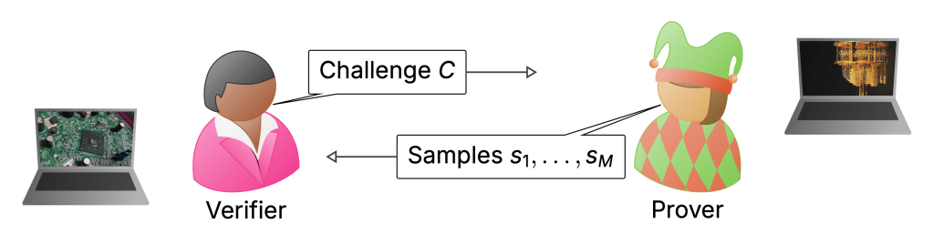
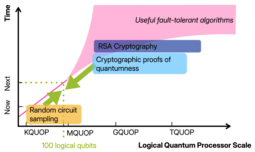
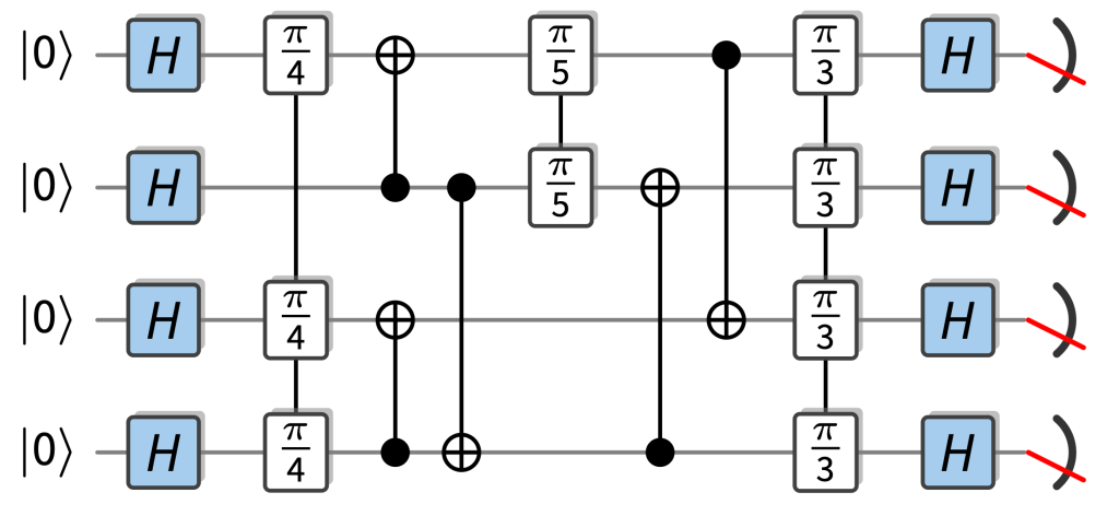
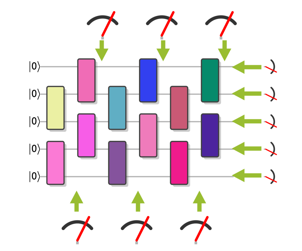

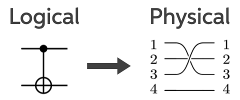
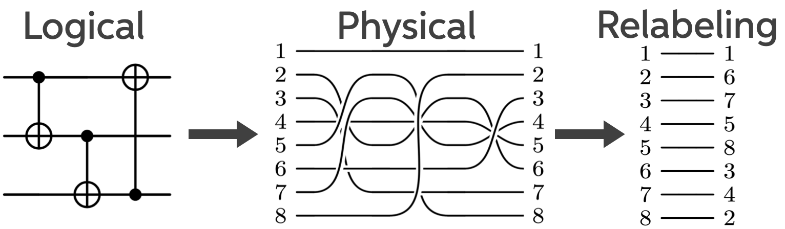
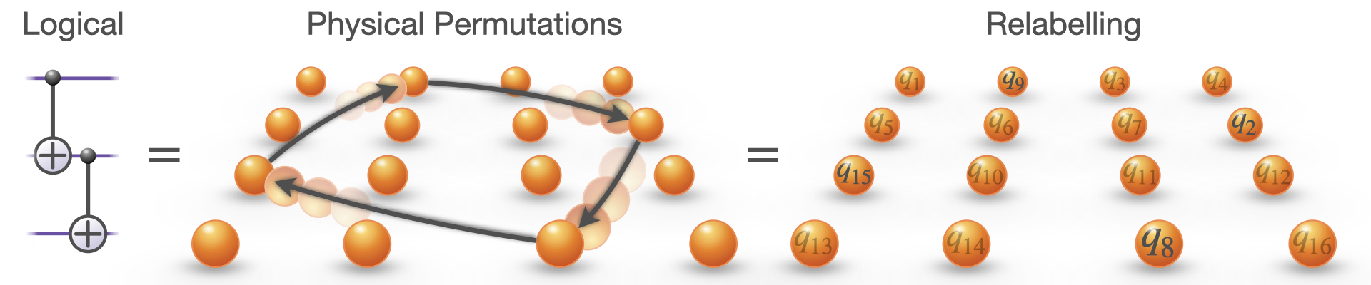
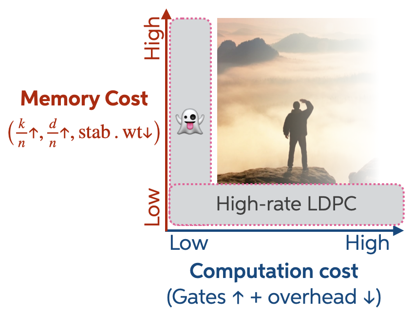
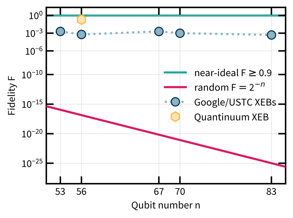
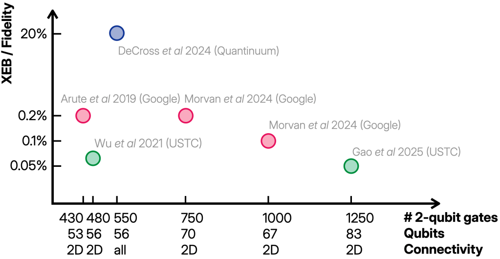

 minutes, Interviewer #2 and I could scarcely make each other’s acquaintance. So I smuggled travel time into my schedule.

 and
and  —addressing directly the extent of topological protection of the states generated by non-Abelian anyons. Behavior clearly conforming to the trends highlighted above could certify the device as a topological quantum memory. (Personally, I most anxiously await this milestone.)
