
Last Monday was an exciting day!
After following the BICEP2 announcement via Twitter, I had to board a transcontinental flight, so I had 5 uninterrupted hours to think about what it all meant. Without Internet access or references, and having not thought seriously about inflation for decades, I wanted to reconstruct a few scraps of knowledge needed to interpret the implications of r ~ 0.2.
I did what any physicist would have done … I derived the basic equations without worrying about niceties such as factors of 3 or 
By tradition, careless estimates like these are called “back-of-the-envelope” calculations. There have been times when I have made notes on the back of an envelope, or a napkin or place mat. But in this case I had the presence of mind to bring a notepad with me.

Notes from a plane ride
According to inflation theory, a nearly homogeneous scalar field called the inflaton (denoted by 

Gradually, the rolling inflaton picked up speed. When its kinetic energy became comparable to its potential energy, inflation ended, and the universe “reheated” — the energy previously stored in the potential
Both the density perturbations and the gravitational waves have been detected via their influence on the inhomogeneities in the cosmic microwave background. The 2.726 K photons left over from the big bang have a nearly uniform temperature as we scan across the sky, but there are small deviations from perfect uniformity that have been precisely measured. We won’t worry about the details of how the size of the perturbations is inferred from the data. Our goal is to achieve a crude understanding of how the density perturbations and gravitational waves are related, which is what the BICEP2 results are telling us about. We also won’t worry about the details of the shape of the potential function
Exponential expansion
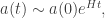
Einstein’s field equations tell us how the rate at which the universe expands during inflation is related to energy density stored in the scalar field potential. If a(t) is the “scale factor” which describes how lengths grow with time, then roughly

Here 


(To persuade yourself that this is at least roughly the right equation, you should note that a similar equation applies to an expanding spherical ball of radius a(t) with uniform mass density V. But in the case of the ball, the mass density would decrease as the ball expands. The universe is different — it can expand without diluting its mass density, so the rate of expansion 
During inflation, the scalar field 
where 

To explain the smoothness of the observed universe, we require at least 50 “e-foldings” of inflation before the universe reheated — that is, inflation should have lasted for a time at least 
Slow rolling
During inflation the inflaton 

Here 
Density perturbations
The trickiest thing we need to understand is how inflation produced the density perturbations which later seeded the formation of galaxies. There are several steps to the argument.
Quantum fluctuations of the inflaton
As the universe inflates, the inflaton field is subject to quantum fluctuations, where the size of the fluctuation depends on its wavelength. Due to inflation, the wavelength increases rapidly, like 

Well, first of all, how big are the fluctuations when they leave the horizon during inflation? Then the wavelength is

From inflaton fluctuations to density perturbations
Reheating occurs abruptly when the inflaton field reaches a particular value. Because of the quantum fluctuations, some horizon volumes have larger than average values of
When we compare different regions of comparable size, we can find the typical (root-mean-square) fluctuations 

Small fractional fluctuations in the scale factor 


The subscript hor serves to remind us that this is the size of density perturbations as they cross the horizon, before they get a chance to grow due to gravitational instabilities. We have found our first important conclusion: The density perturbations have a size determined by the Hubble constant 

Perturbations in terms of the potential
Putting together 

The observed density perturbations are telling us something interesting about the scalar field potential during inflation.
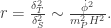
Gravitational waves and the meaning of r
The gravitational field as well as the inflaton field is subject to quantum fluctuations during inflation. We call these tensor fluctuations to distinguish them from the scalar fluctuations in the energy density. The tensor fluctuations have an effect on the microwave anisotropy which can be distinguished in principle from the scalar fluctuations. We’ll just take that for granted here, without worrying about the details of how it’s done.
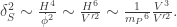
While a scalar field fluctuation with wavelength 


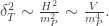
From observations of the CMB anisotropy we know that 

is about 

This is our second important conclusion: The energy density during inflation defines a mass scale, which turns our to be 

Rolling, rolling, rolling, …
Using 
It is convenient to measure time in units of the number 

Now, we know that for inflation to explain the smoothness of the universe we need 

This is our third important conclusion — the inflaton field had to roll a long, long, way during inflation — it changed by much more than the Planck scale! Putting in the O(1) factors we have left out reduces the required amount of rolling by about a factor of 3, but we still conclude that the rolling was super-Planckian if
Spectral tilt
As the inflaton rolls, the potential energy, and hence also the Hubble constant
To keep things simple, let’s suppose that the rate of rolling is constant during inflation, at least over the length scales for which we have data. Using 
Using 
From 

and using 

Putting in the numbers more carefully we find a scalar spectral tilt of 

This is our last important conclusion: A relatively large value of 
Summing up
If you have stuck with me this far, and you haven’t seen this stuff before, I hope you’re impressed. Of course, everything I’ve described can be done much more carefully. I’ve tried to convey, though, that the emerging story seems to hold together pretty well. Compared to last week, we have stronger evidence now that inflation occurred, that the mass scale of inflation is high, and that the scalar and tensor fluctuations produced during inflation have been detected. One prediction is that the tensor fluctuations, like the scalar ones, should have a notable spectral tilt, though a lot more data will be needed to pin that down.
I apologize to the experts again, for the sloppiness of these arguments. I hope that I have at least faithfully conveyed some of the spirit of inflation theory in a way that seems somewhat accessible to the uninitiated. And I’m sorry there are no references, but I wasn’t sure which ones to include (and I was too lazy to track them down).
It should also be clear that much can be done to sharpen the confrontation between theory and experiment. A whole lot of fun lies ahead.
Added notes (3/25/2014):
Okay, here’s a good reference, a useful review article by Baumann. (I found out about it on Twitter!)
From Baumann’s lectures I learned a convenient notation. The rolling of the inflaton can be characterized by two “potential slow-roll parameters” defined by

Both parameters are small during slow rolling, but the relationship between them depends on the shape of the potential. My crude approximation (
We can express the spectral tilt (as I defined it) in terms of these parameters, finding 


keeping factors of 3 that I left out before. (As a homework exercise, check these formulas for the tensor and scalar tilt.)
It is also easy to see that 

We see, though, that the conclusion that the tensor tilt is
Once again, we’re lucky. On the one hand, it’s good to have a robust prediction (for the tensor tilt). On the other hand, it’s good to have a handle (the scalar tilt) for distinguishing among different inflationary models.
One last point is worth mentioning. We have set Planck’s constant 

Thus the production of gravitational waves during inflation is a quantum effect, which would disappear in the limit 

Therefore the detection of primordial gravitational waves by BICEP2, if correct, confirms that gravity is quantized just like the other fundamental forces. That shouldn’t be a surprise, but it’s nice to know.

thanks for this succinct account..i have been looking for something like this for sometime and all i got were tediums of jargon and calculations..
Question: How many assumptions including numbers like the strenghth of the inflaton field did yo put in by hand into your calculations to reproduce how many observational facts?
The story is not overwhelmingly impressive from that point of view, although it’s encouraging that the observed value of r seems to fit together reasonably well with the observed scalar spectral tilt. The more relevant question, I think, is whether the signal detected by BICEP2 is really of cosmological origin, and if so whether there is any reasonable explanation other than gravitational waves produced during inflation. When other experiments see the signal at other frequencies we’ll be more convinced about the first point, and meanwhile theorists will be working hard to address the second point.
“Compared to last week, we have strong evidence now that inflation occurred …” My impression is that even before the BICEP2 results, Linde claimed that inflation (in some form, at least) had been proven beyond a reasonable doubt. Also, Witten has been convinced for many years that inflation occurred. The inflation theories of Guth, Linde, et al. imply that Newton-Einstein gravitational theory is 100% correct, apparently contradicting Milgrom’s acceleration law.
On 14 March 2014 Kroupa wrote, “The falsification of the standard model of cosmology (to be more precise, of the existence of cold or warm dark matter particles) is very robust indeed. It is completely consistent with all existing data.”
http://www.scilogs.com/the-dark-matter-crisis/2013/11/22/pavel-kroupa-on-the-vast-polar-structures-around-the-milky-way-and-andromeda/
I conjecture that the inflation theories of Guth, Linde, et al. will find it very difficult to explain the space roar. In my theory, inflation is due to a statistically significant escape of gravitons from the boundary of the multiverse into the interior of the multiverse, and the space roar is entirely due to electromagnetic radiation emitted by the inflaton field. My guess is that Linde’s theory of chaotic inflation is correct if and only if dark matter particles exist.
Pingback: Inflation on the back of an envelope | Φ&up...
I’m guessing that when all of the matter in the universe is in one place the gravitational force has defeated all the other forces of nature; locked them up and thrown away the key. Maybe that kind of reality is a big casino with an infinite number of slot machines. If the right numbers come up on any machine the other forces get a get out of jail card. But, in lieu of that, what force could possible push back against the force of gravity in that state?
Pingback: Allgemeines Live-Blog ab dem 22. März 2014 | Skyweek Zwei Punkt Null
“What inhomogeneities remained arose from quantum fluctuations in the inflaton and the spacetime geometry occurring during the inflationary period.” The preceding statement should be true in both Newton-Einstein inflation and Milgrom inflation.
“Einstein’s field equations tell us how the rate at which the universe expands during inflation is related to energy density stored in the scalar field potential.” The preceding statement is true in Newton-Einstein inflation but might not be true in Milgrom inflation.
What is the simplest way that Einstein’s field equations might fail? Replace the -1/2 in the standard form of Einstein’s field equations by -1/2 + dark-matter-compensation-constant. This idea might not work. However, in any case, my guess is that Milgrom is the Kepler of contemporary cosmology. I also guess that the main problem with string theory is that string theorists fail to realize that Milgrom is the Kepler of contemporary cosmology. Are string vibrations confined to 3 copies of the Leech lattice? Perhaps not. However, I predict that the inflation theories of Guth, Linde, et al. are not quite correct, because these theories are incompatible with Milgromian dynamics.
Thank you for showing your actual “back of the envelope.” It brought back memories of Ed Purcell teaching E&M (“Physics 12B”) in the spring of 1976. One day the class laughed when Ed set c=1 and e=1 and pi=1 to do an order-of-magnitude calculation. Ed turned from the board surprised and a bit crestfallen, sharing with the class that “until you are able to back-of-the-envelope calculations, you are not ready to do physics.” The next class Ed actually brought in an envelope and an overhead projector, and he taught that day’s class by writing on the envelope rather than on the blackboard. I can’t remember who the TA was in 1976 (he was also an outstanding teacher), but Ed’s passion for order-of-magnitude calculations remains indelible. The notes from your airplane trip are very much in this spirit.
Pingback: B-mode News | Not Even Wrong
What a nice, clear, interesting post…
Dear John,
Thank you for the nice summary and the calculations. It does give a good overview to non-specialists.
However, I wonder if one can really deduce anything about the quantization of the gravitational waves. The model you presented does assume that the fluctuations are quantum, but could there be a model with just classical fluctuations which may have produced the same B-mode pattern? While the current predictions are consistent with a quantum model, they may also be consistent with some classical model as well. The classical model might need some strange initial stochastic fluctuations to reproduce the observed pattern, but maybe these can be reasonably assumed for the very early stages of the universe. Or can it be said without reasonable doubt that all meaningful classical models are excluded? And if so, why?
I don’t know a plausible classical explanation for the origin of the gravitational waves. It’s a good problem to search for one.
Is ‘t Hooft determinism the best hope for a model of deterministic origin for gravitational waves? Is Newton-Einstein inflation versus Milgrom inflation the key to understanding ‘t Hooft determinism?
http://arxiv.org/abs/1207.3612 “Discreteness and Determinism in Superstrings” by Gerard ‘t Hooft, 2012
VIEWPOINT 1: Classical reality is an approximation to quantum reality. Measurement modifies quantum reality.
VIEWPOINT 2: Classical reality is an approximation to quantum reality, and quantum reality is an approximation generated by Wolfram’s automaton. Measurement is a natural process that creates quantum reality using 3 copies of the Leech lattice and Fredkin-Wolfram information below the Planck scale. String vibrations are confined to 3 copies of the Leech lattice, and this confinement enables string theory to make testable predictions by means of ‘t Hooft determinism.
Pingback: O Futuro da Cosmologia pós BICEP2 | True Singularity
Reblogged this on The truth is in the details.
Pingback: Intelligent Design a Nobel Prize ~ The Importance of Asymmetry and How Einstein Made Asymmetry, the AEther, the Atma, and the Swastika Disappear | Alternative Thinking 37
Pingback: 'There shall be reheating' and other inflation-related questions - FAQs System
What do you think of physics-by-press-conference? I recall Caltech being involved in the reaction to Pons-Fleischmann, so many years ago. Now it looks like my dear alma mater is on the other side of the bar re BICEP2. V painful to observe…
fast forward to Spring of ’15
Pingback: BICEP2 Redux: How the Sausage is Made | Whiskey…Tango…Foxtrot?
Pingback: To become a good teacher, ignore everything you’re told and learn from the masters (part 4 of 4) | Quantum Frontiers
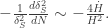
I was wondering if you have a reference for your formula that the spectral tilt =- \frac{1}{\delta^2_s} \frac{d \delta^2_s}{d N}. I have only seen it in other places defined in terms of k but I would like to use it in this form.