Has quantum advantage been achieved? Part 2: Considering the evidence

Posted on January 25, 2026 by Dominik Hangleiter

Welcome back to: Has quantum advantage been achieved?

In Part 1 of this mini-series on quantum advantage demonstrations, I told you about the idea of random circuit sampling (RCS) and the experimental implementations thereof. In this post, Part 2 out of 3, I will discuss the arguments and evidence for why I am convinced that the experiments demonstrate a quantum advantage.

Recall from Part 1 that to assess an experimental quantum advantage claim we need to check three criteria:

Does the experiment correctly solve a computational task?
Does it achieve a scalable advantage over classical computation?
Does it achieve an in-practice advantage over the best classical attempt at solving the task?

What’s the issue?

When assessing these criteria for the RCS experiments there is an important problem: The early quantum computers we ran them on were very far from being reliable and the computation was significantly corrupted by noise. How should we interpret this noisy data? Or more concisely:

Is random circuit sampling still classically hard even when we allow for whatever amount of noise the actual experiments had?
Can we be convinced from the experimental data that this task has actually been solved?

I want to convince you today that we have developed a very good understanding of these questions that gives a solid underpinning to the advantage claim. Developing that understanding required a mix of methodologies from different areas of science, including theoretical computer science, algorithm design, and physics and has been an exciting journey over the past years.

The noisy sampling task

Let us start by answering the base question. What computational task did the experiments actually solve?

Recall that, in the ideal RCS scenario, we are given a random circuit $C$ on $n$ qubits and the task is to sample from the output distribution of the state obtained $\ket C$ from applying the circuit $C$ to a simple reference state. The output probability distribution of this state is determined by the Born rule when I measure every qubit in a fixed choice of basis.

Now what does a noisy quantum computer do when I execute all the gates on it and apply them to its state? Well, it prepares a noisy version $\rho_ C$ of the intended state $\ket C$ and once I measure the qubits, I obtain samples from the output distribution of that noisy state.

We should not make the task dependent on the specifics of that state or the noise that determined it, but we can define a computational task based on this observation by fixing how accurate that noisy state preparation is. The natural way to do this is to use the fidelity

$F(C) = \bra C \rho_C \ket C,$

which is just the overlap between the ideal state and the noisy state. The fidelity is 1 if the noisy state is equal to the ideal state, and 0 if it is perfectly orthogonal to it.

Finite-fidelity random circuit sampling
Given a typical random circuit $C$ , sample from the output distribution of any quantum state whose fidelity with the ideal output state $\ket C$ is at least $\delta$ .

Note that finite-fidelity RCS does not demand success for every circuit, but only for typical circuits from the random circuit ensemble. This matches what the experiments do: they draw random circuits and need the device to perform well on the overwhelming majority of those draws. Accordingly, when the experiments quote a single number as “fidelity”, it is really the typical (or, more precisely, circuit-averaged) fidelity that I will just call $F$ .

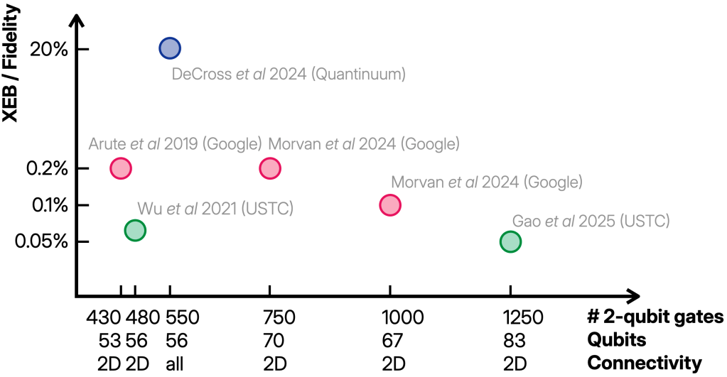
The noisy experiments claim to have solved finite-fidelity RCS for values of $\delta$ around 0.1%. What is more, they consistently achieve this value even as the circuit sizes are increased in the later experiments. Both the actual value and the scaling will be important later.

What is the complexity of finite-fidelity RCS?

Quantum advantage of finite-fidelity RCS

Let’s start off by supposing that the quantum computation is (nearly) perfectly executed, so the required fidelity $\delta$ is quite large, say, 90%. In this scenario, we have very good evidence based on computational complexity theory that there is a scalable and in-practice quantum advantage for RCS. This evidence is very strong, comparable to the evidence we have for the hardness of factoring and simulating quantum systems. The intuition behind it is that quantum output probabilities are extremely hard to compute because of a mechanism behind quantum advantages: destructive interference. If you are interested in the subtleties and the open questions, take a look at our survey.

The question is now, how far down in fidelity this classical hardness persists? Intuitively, the smaller we make $\delta$ , the easier finite-fidelity RCS should become for a classical algorithm (and a quantum computer, too), since the freedom we have in deviating from the ideal state in our simulation becomes larger and larger. This increases the possibility of finding a state that turns out to be easy to simulate within the fidelity constraint.

Somewhat surprisingly, though, finite-fidelity RCS seems to remain hard even for very small values of $\delta$ . I am not aware of any efficient classical algorithm that achieves the finite-fidelity task for $\delta$ significantly away from the baseline trivial value of $2^{-n}$ . This is the value a maximally mixed or randomly picked state achieves because a random state has no correlation with the ideal state (or any other state), and $2^{-n}$ is exactly what you expect in that case (while 0 would correspond to perfect anti-correlation).

One can save some classical runtime compared to solving near-ideal RCS by exploiting a reduced fidelity, but the costs remain exponential. To classically solve finite-fidelity RCS, the best known approaches are reported in the papers that performed classical simulations of finite-fidelity RCS with the parameters of the first Google and USTC experiment (classSim1, classSim2). To achieve this, however, they needed to approximately simulate the ideal circuits at an immense cost. To the best of my knowledge, all but those first two experiments are far out of reach for these algorithms.

Getting the scaling right: weak noise and low depth

So what is the right value of $\delta$ at which we can hope for a scalable and in-practice advantage of RCS experiments?

When thinking about this question, it is helpful to keep a model of the circuit in mind that a noisy experiment runs. So, let us consider a noisy circuit on $n$ qubits with $d$ layers of gates and single-qubit noise of strength $\varepsilon$ on every qubit in every layer. In this scenario, the typical fidelity with the ideal state will decay as $F \sim \exp(- \varepsilon n d)$ .

Any reasonably testable value of the fidelity needs to scale as $1/\mathsf{poly}(n)$ , since eventually we need to estimate the average fidelity $F$ from the experimental samples and this typically requires at least $1/F^2$ samples, so exponentially small fidelities are experimentally invisible. The polynomial fidelity $\delta$ is also much closer to the near-ideal scenario ( $\delta \geq$ 90%) than the trivial scenario ( $\delta = 2^{-n}$ ). While we cannot formally pin this down, the intuition behind the complexity-theoretic evidence for the hardness of near-ideal RCS persists into the $\delta \sim 1/\mathsf{poly}(n)$ regime: to sample up to such high precision, we still need a reasonably accurate estimate of the ideal probabilities, and getting this is computationally extremely difficult. Scalable quantum advantage in this regime is therefore a pretty safe bet.

How do the parameters of the experiment and the RCS instances need to scale with the number of qubits $n$ to experimentally achieve the fidelity regime? The limit to consider is one in which the noise rate decreases with the number of qubits, while the circuit depth is only allowed to increase very slowly. It depends on the circuit architecture, i.e., the choice of circuit connectivity, and the gate set, through a constant $c_A$ as I will explain in more detail below.

Weak-noise and low-depth scaling
(Weak noise) The local noise rate of the quantum device scales as $\varepsilon \lt c_A/n$ .
(Low depth) The circuit depth scales as $d \lesssim \log n$ .

This limit is such that we have a scaling of the fidelity as $F \gtrsim n^{-c}$ for some constant $c$ . It is also a natural scaling limit for noisy devices whose error rates gradually improve through better engineering. You might be worried about the fact that the depth needs to be quite low but it turns out that there is a solid quantum advantage even for $\log(n)$ -depth circuits.

The precise definition of the weak-noise regime is motivated by the following observation. It turns out to be crucial for assessing the noisy data from the experiment.

Fidelity versus XEB: a phase transition

Remember from Part 1 that the experiments measured a quantity called the cross-entropy benchmark (XEB)

$\chi = 2^{2n} \mathbb E_C \mathbb E_{x} p_C(x) -1 ,$

The XEB averages the ideal probabilities $p_C(x)$ corresponding to the sampled outcomes $x$ from experiments on random circuits $C$ . Thus, it correlates the experimental and ideal output distributions of those random circuits. You can think of it as a “classical version” of the fidelity: If the experimental distribution is correct, the XEB will essentially be 1. If it is uniformly random, the XEB is 0.

The experiments claimed that the XEB is a good proxy for the circuit-averaged fidelity given by $F = \mathbb E_C F(C)$ , and so we need to understand when this is true. Fortunately, in the past few years, alongside with the improved experiments, we have developed a very good understanding of this question (WN, Spoof2, PT1, PT2).

It turns out that the quality of correspondence between XEB and average fidelity depends strongly on the noise in the experimental quantum state. In fact, there is a sharp phase transition: there is an architecture-dependent constant $c_A$ such that when the experimental local noise rate $\varepsilon < c_A/n$ , then the XEB is a good and reliable proxy for the average fidelity for any system size $n$ and circuit depth $d$ . This is exactly the weak-noise regime. Above that threshold, in the strong noise regime, the XEB is an increasingly bad proxy for the fidelity (PT1, PT2).

Let me be more precise: In the weak-noise regime, when we consider the decay of the XEB as a function of circuit depth $d$ , the rate of decay is given by $\varepsilon n$ , i.e., the XEB decays as $\exp(- \varepsilon n d )$ . Meanwhile, in the strong-noise regime the rate of decay is constant, giving an XEB decay as $\exp(- C d)$ for a constant $C$ . At the same time, the fidelity decays as $\exp(- \varepsilon n d )$ regardless of the noise regime. Hence, in the weak-noise regime, the XEB is a good proxy of the fidelity, while in the strong noise regime, there is an exponentially increasing gap between the XEB (which remains large) and the fidelity (which continues to decay exponentially). regardless of the noise regime.

This is what the following plot shows. We computed it from an exact mapping of the behavior of the XEB to the dynamics of a statistical-mechanics model that can be evaluated efficiently. Using this mapping, we can also compute the noise threshold $c_A$ for whichever random circuit family and architecture you are interested in.

From (PT2). The $y$ -axis label $\Delta( \ln \chi )$ is the decay rate of the XEB $\chi$ , $N=n$ the number of qubits and $\varepsilon$ is the local noise rate.

Where are the experiments?

We are now ready to take a look at the crux when assessing the noisy data: Can we trust the reported XEB values as an estimator of the fidelity? If so, do the experiments solve finite-fidelity RCS in the solidly hard regime where $\delta \geq 1/ \mathsf{poly}(n)$ ?

In their more recent paper (PT1), the Google team explicitly verified that the experiment is well below the phase transition, and it turns out that the first experiment was just at the boundary. The USTC experiments had comparable noise rates, and the Quantinuum experiment much better ones. Since fidelity decays as $\exp(-\varepsilon n d)$ , but the reported XEB values stayed consistently around 0.1% as $n$ was increased, the experimental error rate $\varepsilon$ of the experiments improved even better than the $1/n$ scaling required for the weak-noise regime, namely, more like $\varepsilon \sim 1/(nd)$ . Altogether, the experiments are therefore in the weak-noise regime both in terms of absolute numbers relative to $c_A/n$ and the required scaling.

Of course, to derive the transition, we made some assumptions about the noise such as that the noise is local, and that it does not depend much on the circuit itself. In the advantage experiments, these assumptions about the noise are characterized and tested. This is done through a variety of means at increasing levels of complexity, including detailed characterization of the noise in individual gates, gates run in parallel, and eventually in a larger circuit. The importance of understanding the noise shows in the fact that a significant portion of the supplementary materials of the advantage experiments is dedicated to getting this right. All of this contributes to the experimental justification for using the XEB as a proxy for the fidelity!

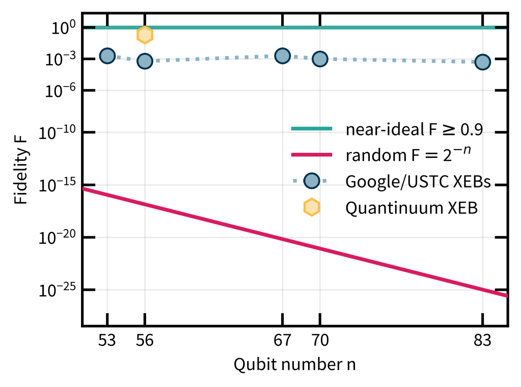
The data shows that the experiments solved finite-fidelity RCS for values of $\delta$ above the constant value of roughly 0.1% as the experiments grew. In the following plot, I compare the experimental fidelity values to the near-ideal scenario on the one hand, and the trivial $2^{-n}$ value on the other hand. Viewed at this scale, the values of $\delta$ for which the experiment solved finite-fidelity RCS are indeed vastly closer to the near-ideal value than the trivial baseline, which should boost our confidence that reproducing samples at a similar fidelity is extremely challenging.

The phase transition matters!

You might be tempted to say: “Well, but is all this really so important? Can’t I just use XEB and forget all about fidelity?”

The phase transition shows why that would change the complexity of the problem: in the strong-noise regime, XEB can stay high even when fidelity is exponentially small. And indeed, this discrepancy can be exploited by so-called spoofers for the XEB. These are efficient classical algorithms which can be used to succeed at a quantum advantage test even though they clearly do not achieve the intended advantage. These spoofers (Spoof1, Spoof2) can achieve high XEB scores comparable to those of the experiments and scaling like $\exp(-cd)$ in the circuit depth $d$ for some constant $c$ .

Their basic idea is to introduce strong, judiciously chosen noise at specific circuit locations that has the effect of breaking up the simulation task up into smaller, much easier components, but at the same time still gives a high XEB score. In doing so, they exploit the strong-noise regime in which the XEB is a really bad proxy for the fidelity. This allows them to sample from states with exponentially low fidelity while achieving a high XEB value.

The discovery of the phase transition and the associated spoofers highlights the importance of modeling when assessing—and even formulating—the advantage claim based on noisy data.

But we can’t compute the XEB!

You might also be worried that the experiments did not actually compute the XEB in the advantage regime because to estimate it they would have needed to compute ideal probabilities—a task that is hard by definition of the advantage regime. Instead, they used a bunch of different ways to extrapolate the true XEB from XEB proxies (proxy of a proxy of the fidelity). Is this is a valid way of getting an estimate of the true XEB?

It totally is! Different extrapolations—from easy-to-simulate to hard-to-simulate, from small system to large system etc—all gave consistent answers for the experimental XEB value of the supremacy circuits. Think of this as having several lines that cross in the same point. For that crossing to be a coincidence, something crazy, conspiratorial must happen exactly when you move to the supremacy circuits from different directions. That is why it is reasonable to trust the reported value of the XEB.

That’s exactly how experiments work!

All of this is to say that establishing that the experiments correctly solved finite-fidelity RCS and therefore show quantum advantage involved a lot of experimental characterization of the noise as well as theoretical work to understand the effects of noise on the quantity we care about—the fidelity between the experimental and ideal states.

In this respect (and maybe also in the scale of the discovery), the quantum advantage experiments are similar to the recent experiments reporting discovery of the Higgs boson and gravitational waves. While I do not claim to understand any of the details, what I do understand is that in both experiments, there is an unfathomable amount of data that could not be interpreted without preselection and post-processing of the data, theories, extrapolations and approximations that model the experiment and measurement apparatus. All of those enter the respective smoking-gun plots that show the discoveries.

If you believe in the validity of experimental physics methodology, you should therefore also believe in the type of evidence underlying experimental claim of the quantum advantage demonstrations: that they sampled from the output distribution of a quantum state with the reported fidelities.

Put succinctly: If you believe in the Higgs boson and gravitational waves, you should probably also believe in the experimental demonstration of quantum advantage.

What are the counter-arguments?

The theoretical computer scientist

“The weak-noise limit is not physical. The appropriate scaling limit is one in which the local noise rate of the device is constant while the system size grows, and in that case, there is a classical simulation algorithm for RCS (SimIQP, SimRCS).”

In theoretical computer science, scaling of time or the system size in the input size is considered very natural: We say an algorithm is efficient if its runtime and space usage only depend polynomially on the input size.

But all scaling arguments are hypothetical concepts, and we only care about the scaling at relevant sizes. In the end, every scaling limit is going to hit the wall of physical reality—be it the amount of energy or human lifetime that limits the time of an algorithm, or the physical resources that are required to build larger and larger computers. To keep the scaling limit going as we increase the size of our computations, we need innovation that makes the components smaller and less noisy.

At the scales relevant to RCS, the $1/n$ scaling of the noise is benign and even natural. Why? Well, currently, the actual noise in quantum computers is not governed by the fundamental limit, but by engineering challenges. Realizing this limit therefore amounts to engineering improvements in the system size and noise rate that are achieved over time. Sure, at some point that scaling limit is also going to hit a fundamental barrier below which the noise cannot be improved. But we are surely far away from that limit, yet. What is more, already now logical qubits are starting to work and achieve beyond-breakeven fidelities. So even if the engineering improvements should flatten out from here onward, QEC will keep the $1/n$ noise limit going and even accelerate it in the intermediate future.

The complexity maniac

“All the hard complexity-theoretic evidence for quantum advantage is in the near-ideal regime, but now you are claiming advantage for the low-fidelity version of that task.”

This is probably the strongest counter-argument in my opinion, and I gave my best response above. Let me just add that this is a question about computational complexity. In the end, all of complexity theory is based on belief. The only real evidence we have for the hardness of any task is the absence of an efficient algorithm, or the reduction to a paradigmatic, well-studied task for which there is no efficient algorithm.

I am not sure how much I would bet that you cannot find an efficient algorithm for finite-fidelity RCS in the regime of the experiments, but it is certainly a pizza.

The enthusiastic skeptic

“There is no verification test that just depends on the classical samples, is efficient and does not make any assumptions about the device. In particular, you cannot unconditionally verify fidelity just from the classical samples. Why should I believe the data?”

Yes, sure, the current advantage demonstrations are not device-independent. But the comparison you should have in mind are Bell tests. The first proper Bell tests of Aspect and others in the 80s were not free of loopholes. They still allowed for contrived explanations of the data that did not violate local realism. Still, I can hardly believe that anyone would argue that Bell inequalities were not violated already back then.

As the years passed, these remaining loopholes were closed. To be a skeptic of the data, people needed to come up with more and more adversarial scenarios that could explain the data. We are working on the same to happen with quantum advantage demonstrations: come up with better schemes and better tests that require less and less assumptions or knowledge about the specifics of the device.

The “this is unfair” argument

“When you chose the gates and architecture of the circuit dependent on your device, you tailored the task too much to the device and that is unfair. Not even the different RCS experiments solve exactly the same task.”

This is not really an argument against the achievement of quantum advantage but more against the particular choices of circuit ensembles in the experiments. Sure, the specific computations solved are still somewhat tailored to the hardware itself and in this sense the experiments are not hardware-independent yet, but they still solve fine computational tasks. Moving away from such hardware-tailored task specifications is another important next step and we are working on it.

In the third and last part of this mini series I will address next steps in quantum advantage that aim at closing some of the remaining loopholes. The most important—and theoretically interesting—one is to enable efficient verification of quantum advantage using less or even no specific knowledge about the device that was used, but just the measurement outcomes.

References

(survey) Hangleiter, D. & Eisert, J. Computational advantage of quantum random sampling. Rev. Mod. Phys. 95, 035001 (2023).

(classSim1) Pan, F., Chen, K. & Zhang, P. Solving the sampling problem of the Sycamore quantum circuits. Phys. Rev. Lett. 129, 090502 (2022).

(classSim2) Kalachev, G., Panteleev, P., Zhou, P. & Yung, M.-H. Classical Sampling of Random Quantum Circuits with Bounded Fidelity. arXiv.2112.15083 (2021).

(WN) Dalzell, A. M., Hunter-Jones, N. & Brandão, F. G. S. L. Random Quantum Circuits Transform Local Noise into Global White Noise. Commun. Math. Phys. 405, 78 (2024).

(PT1)vMorvan, A. et al. Phase transitions in random circuit sampling. Nature 634, 328–333 (2024).

(PT2) Ware, B. et al. A sharp phase transition in linear cross-entropy benchmarking. arXiv:2305.04954 (2023).

(Spoof1) Barak, B., Chou, C.-N. & Gao, X. Spoofing Linear Cross-Entropy Benchmarking in Shallow Quantum Circuits. in 12th Innovations in Theoretical Computer Science Conference (ITCS 2021) (ed. Lee, J. R.) vol. 185 30:1-30:20 (2021).

(Spoof2) Gao, X. et al. Limitations of Linear Cross-Entropy as a Measure for Quantum Advantage. PRX Quantum 5, 010334 (2024).

(SimIQP) Bremner, M. J., Montanaro, A. & Shepherd, D. J. Achieving quantum supremacy with sparse and noisy commuting quantum computations. Quantum 1, 8 (2017).

(SimRCS) Aharonov, D., Gao, X., Landau, Z., Liu, Y. & Vazirani, U. A polynomial-time classical algorithm for noisy random circuit sampling. in Proceedings of the 55th Annual ACM Symposium on Theory of Computing 945–957 (2023).

Has quantum advantage been achieved?

Posted on January 6, 2026 by Dominik Hangleiter

Recently, I gave a couple of perspective talks on quantum advantage, one at the annual retreat of the CIQC and one at a recent KITP programme. I started off by polling the audience on who believed quantum advantage had been achieved. Just this one, simple question.

The audience was mostly experimental and theoretical physicists with a few CS theory folks sprinkled in. I was sure that these audiences would be overwhelmingly convinced of the successful demonstration of quantum advantage. After all, more than half a decade has passed since the first experimental claim (G1) of “quantum supremacy” as the patron of this blog’s institute called the idea “to perform tasks with controlled quantum systems going beyond what can be achieved with ordinary digital computers” (Preskill, p. 2) back in 2012. Yes, this first experiment by the Google team may have been simulated in the meantime, but it was only the first in an impressive series of similar demonstrations that became bigger and better with every year that passed. Surely, so I thought, a significant part of my audiences would have been convinced of quantum advantage even before Google’s claim, when so-called quantum simulation experiments claimed to have performed computations that no classical computer could do (e.g. (qSim)).

I could not have been more wrong.

In both talks, less than half of the people in the audience thought that quantum advantage had been achieved.

In the discussions that ensued, I came to understand what folks criticized about the experiments that have been performed and even the concept of quantum advantage to begin with. But more on that later. Most of all, it seemed to me, the community had dismissed Google’s advantage claim because of the classical simulation shortly after. It hadn’t quite kept track of all the advances—theoretical and experimental—since then.

In a mini-series of three posts, I want to remedy this and convince you that the existing quantum computers can perform tasks that no classical computer can do. Let me caution, though, that the experiments I am going to talk about solve a (nearly) useless task. Nothing of what I say implies that you should (yet) be worried about your bank accounts.

I will start off by recapping what quantum advantage is and how it has been demonstrated in a set of experiments over the past few years.

Part 1: What is quantum advantage and what has been done?

To state the obvious: we are now fairly convinced that noiseless quantum computers would be able solve problems efficiently that no classical computer could solve. In fact, we have been convinced of that already since the mid-90ies when Lloyd and Shor discovered two basic quantum algorithms: simulating quantum systems and factoring large numbers. Both of these are tasks where we are as certain as we could be that no classical computer can solve them. So why talk about quantum advantage 20 and 30 years later?

The idea of a quantum advantage demonstration—be it on a completely useless task even—emerged as a milestone for the field in the 2010s. Achieving quantum advantage would finally demonstrate that quantum computing was not just a random idea of a bunch of academics who took quantum mechanics too seriously. It would show that quantum speedups are real: We can actually build quantum devices, control their states and the noise in them, and use them to solve tasks which not even the largest classical supercomputers could do—and these are very large.

What is quantum advantage?

But what exactly do we mean by “quantum advantage”. It is a vague concept, for sure. But some essential criteria that a demonstration should certainly satisfy are probably the following.

The quantum device needs to solve a pre-specified computational task. This means that there needs to be an input to the quantum computer. Given the input, the quantum computer must then be programmed to solve the task for the given input. This may sound trivial. But it is crucial because it delineates programmable computing devices from just experiments on any odd physical system.
There must be a scaling difference in the time it takes for a quantum computer to solve the task and the time it takes for a classical computer. As we make the problem or input size larger, the difference between the quantum and classical solution times should increase disproportionately, ideally exponentially.
And finally: the actual task solved by the quantum computer should not be solvable by any classical machine (at the time).

Achieving this last criterion using imperfect, noisy quantum devices is the challenge the idea of quantum supremacy set for the field. After all, running any of our favourite quantum algorithms in a classically hard regime on these devices is completely out of the question. They are too small and too noisy. So the field had to come up with the conceivably smallest and most noise-robust quantum algorithm that has a significant scaling advantage against classical computation.

Random circuits are really hard to simulate!

The idea is simple: we just run a random computation, constructed in a way that is as favorable as we can make it to the quantum device while being as hard as possible classically. This may strike as a pretty unfair way to come up with a computational task—it is just built to be hard for classical computers without any other purpose. But: it is a fine computational task. There is an input: the description of the quantum circuit, drawn randomly. The device needs to be programmed to run this exact circuit. And there is a task: just return whatever this quantum computation would return. These are strings of 0s and 1s drawn from a certain distribution. Getting the distribution of the strings right for a given input circuit is the computational task.

This task, dubbed random circuit sampling, can be solved on a classical as well as a quantum computer, but there is a (presumably) exponential advantage for the quantum computer. More on that in Part 2.

For now, let me tell you about the experimental demonstrations of random circuit sampling. Allow me to be slightly more formal. The task solved in random circuit sampling is to produce bit strings $x \in \{0,1\}^n$ distributed according to the Born-rule outcome distribution

$p_C(x) = | \bra x C \ket {0}|^2$

of a sequence of elementary quantum operations (unitary rotations of one or two qubits at a time) which is drawn randomly according to certain rules. This circuit $C$ is applied to a reference state $\ket 0$ on the quantum computer and then measured, giving the string $x$ as an outcome.

The breakthrough: classically hard programmable quantum computations in the real world

In the first quantum supremacy experiment (G1) by the Google team, the quantum computer was built from 53 superconducting qubits arranged in a 2D grid. The operations were randomly chosen simple one-qubit gates ( $\sqrt X, \sqrt Y, \sqrt{X+Y}$ ) and deterministic two-qubit gates called fSim applied in the 2D pattern, and repeated a certain number of times (the depth of the circuit). The limiting factor in these experiments was the quality of the two-qubit gates and the measurements, with error probabilities around 0.6 % and 4 %, respectively.

A very similar experiment was performed by the USTC team on 56 qubits (U1) and both experiments were repeated with better fidelities (0.4 % and 1 % for two-qubit gates and measurements) and slightly larger system sizes (70 and 83 qubits, respectively) in the past two years (G2,U2).

Using a trapped-ion architecture, the Quantinuum team also demonstrated random circuit sampling on 56 qubits but with arbitrary connectivity (random regular graphs) (Q). There, the two-qubit gates were $\pi/2$ -rotations around $Z \otimes Z$ , the single-qubit gates were uniformly random and the error rates much better (0.15 % for both two-qubit gate and measurement errors).

All the experiments ran random circuits on varying system sizes and circuit depths, and collected thousands to millions of samples from a few random circuits at a given size. To benchmark the quality of the samples, the widely accepted benchmark is now the linear cross-entropy (XEB) benchmark defined as

$\chi = 2^{2n} \mathbb E_C \mathbb E_{x} p_C(x) -1 ,$

for an $n$ -qubit circuit. The expectation over $C$ is over the random choice of circuit and the expectation over $x$ is over the experimental distribution of the bit strings. In other words, to compute the XEB given a list of samples, you ‘just’ need to compute the ideal probability of obtaining that sample from the circuit $C$ and average the outcomes.

The XEB is nice because it gives 1 for ideal samples from sufficiently random circuits and 0 for uniformly random samples, and it can be estimated accurately from just a few samples. Under the right conditions, it turns out to be a good proxy for the many-body fidelity of the quantum state prepared just before the measurement.

This tells us that we should expect an XEB score of $(1-\text{error per gate})^{\text{\# gates}} \sim c^{- n d }$ for some noise- and architecture-dependent constant $c$ . All of the experiments achieved a value of the XEB that was significantly (in the statistical sense) far away from 0 as you can see in the plot below. This shows that something nontrivial is going on in the experiments, because the fidelity we expect for a maximally mixed or random state is $2^{-n}$ which is less than $10^{-14}$ % for all the experiments.

The complexity of simulating these experiments is roughly governed by an exponential in either the number of qubits or the maximum bipartite entanglement generated. Figure 5 of the Quantinuum paper has a nice comparison.

It is not easy to say how much leverage an XEB significantly lower than 1 gives a classical spoofer. But one can certainly use it to judiciously change the circuit a tiny bit to make it easier to simulate.

Even then, reproducing the low scores between 0.05 % and 0.2 % of the experiments is extremely hard on classical computers. To the best of my knowledge, producing samples that match the experimental XEB score has only been achieved for the first experiment from 2019 (PCZ). This simulation already exploited the relatively low XEB score to simplify the computation, but even for the slightly larger 56 qubit experiments these techniques may not be feasibly run. So to the best of my knowledge, the only one of the experiments which may actually have been simulated is the 2019 experiment by the Google team.

If there are better methods, or computers, or more willingness to spend money on simulating random circuits today, though, I would be very excited to hear about it!

Proxy of a proxy of a benchmark

Now, you may be wondering: “How do you even compute the XEB or fidelity in a quantum advantage experiment in the first place? Doesn’t it require computing outcome probabilities of the supposedly hard quantum circuits?” And that is indeed a very good question. After all, the quantum advantage of random circuit sampling is based on the hardness of computing these probabilities. This is why, to get an estimate of the XEB in the advantage regime, the experiments needed to use proxies and extrapolation from classically tractable regimes.

This will be important for Part 2 of this series, where I will discuss the evidence we have for quantum advantage, so let me give you some more detail. To extrapolate, one can just run smaller circuits of increasing sizes and extrapolate to the size in the advantage regime. Alternatively, one can run circuits with the same number of gates but with added structure that makes them classically simulatable and extrapolate to the advantage circuits. Extrapolation is based on samples from different experiments from the quantum advantage experiments. All of the experiments did this.

A separate estimate of the XEB score is based on proxies. An XEB proxy uses the samples from the advantage experiments, but computes a different quantity than the XEB that can actually be computed and for which one can collect independent numerical and theoretical evidence that it matches the XEB in the relevant regime. For example, the Google experiments averaged outcome probabilities of modified circuits that were related to the true circuits but easier to simulate.

The Quantinuum experiment did something entirely different, which is to estimate the fidelity of the advantage experiment by inverting the circuit on the quantum computer and measuring the probability of coming back to the initial state.

All of the methods used to estimate the XEB of the quantum advantage experiments required some independent verification based on numerics on smaller sizes and induction to larger sizes, as well as theoretical arguments.

In the end, the advantage claims are thus based on a proxy of a proxy of the quantum fidelity. This is not to say that the advantage claims do not hold. In fact, I will argue in my next post that this is just the way science works. I will also tell you more about the evidence that the experiments I described here actually demonstrate quantum advantage and discuss some skeptical arguments.

Let me close this first post with a few notes.

In describing the quantum supremacy experiments, I focused on random circuit sampling which is run on programmable digital quantum computers. What I neglected to talk about is boson sampling and Gaussian boson sampling, which are run on photonic devices and have also been experimentally demonstrated. The reason for this is that I think random circuits are conceptually cleaner since they are run on processors that are in principle capable of running an arbitrary quantum computation while the photonic devices used in boson sampling are much more limited and bear more resemblance to analog simulators.

I want to continue my poll here, so feel free to write in the comments whether or not you believe that quantum advantage has been demonstrated (by these experiments) and if not, why.

References

[G1] Arute, F. et al. Quantum supremacy using a programmable superconducting processor. Nature 574, 505–510 (2019).

[Preskill] Preskill, J. Quantum computing and the entanglement frontier. arXiv:1203.5813 (2012).

[qSim] Choi, J. et al. Exploring the many-body localization transition in two dimensions. Science 352, 1547–1552 (2016). .

[U1] Wu, Y. et al. Strong Quantum Computational Advantage Using a Superconducting Quantum Processor. Phys. Rev. Lett. 127, 180501 (2021).

[G2] Morvan, A. et al. Phase transitions in random circuit sampling. Nature 634, 328–333 (2024).

[U2] Gao, D. et al. Establishing a New Benchmark in Quantum Computational Advantage with 105-qubit Zuchongzhi 3.0 Processor. Phys. Rev. Lett. 134, 090601 (2025).

[Q] DeCross, M. et al. Computational Power of Random Quantum Circuits in Arbitrary Geometries. Phys. Rev. X 15, 021052 (2025).

[PCZ] Pan, F., Chen, K. & Zhang, P. Solving the sampling problem of the Sycamore quantum circuits. Phys. Rev. Lett. 129, 090502 (2022).

Nicole’s guide to interviewing for faculty positions

Posted on January 4, 2026 by Nicole Yunger Halpern

Snow is haunting weather forecasts, home owners are taking down Christmas lights, stores are discounting exercise equipment, and faculty-hiring committees are winnowing down applications. In-person interviews often take place between January and March but can extend from December to April. If you applied for faculty positions this past fall and you haven’t begun preparing for interviews, begin. This blog post relates my advice about in-person interviews. It most directly addresses assistant professorships in theoretical physics at R1 North American universities, but the advice generalizes to other contexts.

Top takeaway: Your interviewers aim to confirm that they’ll enjoy having you as a colleague. They’ll want to take pleasure in discussing a colloquium with you over coffee, consult you about your area of expertise, take pride in your research achievements, and understand you even if your specialty differs from theirs. You delight in learning and sharing about physics, right? Focus on that delight, and let it shine.

Anatomy of an interview: The typical interview lasts for one or two days. Expect each day to begin between 8:00 and 10:00 AM and to end between 7:00 and 8:30 PM. Yes, you’re justified in feeling exhausted just thinking about such a day. Everyone realizes that faculty interviews are draining, including the people who’ve packed your schedule. But fear not, even if you’re an introvert horrified at the thought of talking for 12 hours straight! Below, I share tips for maintaining your energy level. Your interview will probably involve many of the following components:

One-on-one meetings with faculty members: Vide infra for details and advice.
A meeting with students: Such meetings often happen over lunch or coffee.
Scientific talk: Vide infra.
Chalk talk: Vide infra.
Dinner: Faculty members will typically take you out to dinner. However, as an undergrad, I once joined a student dinner with a faculty candidate. Expect dinner to last a couple of hours, ending between 8:00 and 8:30 PM.
Breakfast: Interviews rarely extend to breakfast, in my experience. But I once underwent an interview whose itinerary was so packed, a faculty member squeezed himself onto the schedule by coming to my hotel’s restaurant for banana bread and yogurt.

After receiving the interview invitation, politely request that your schedule include breaks. First, of course, you’ll thank the search-committee chair (who probably issued the invitation), convey your enthusiasm, and opine about possible interview dates. After accomplishing those tasks, as a candidate, I asked that a 5-to-10-minute break separate consecutive meetings and that 30–45 minutes of quiet time precede my talk (or talks). Why? For two reasons.

First, the search committee was preparing to pack my interview day (or days) to the gills. I’d have to talk for about twelve hours straight. And—much as I adore the physics community, adore learning about physics from colleagues, and adore sharing physics—I’m an introvert. Such a schedule exhausts me. It would probably exhaust all but the world champions of extroversion, and few physicists could even qualify for that competition. After nearly every meeting, I’d find a bathroom, close my eyes, and breathe. (I might also peek at my notes about my next interviewee; vide infra.) The alone time replenished my energy.

Second, committees often schedule interviews back to back. Consecutive interviews might take place in different buildings, though, and walking between buildings doesn’t take zero minutes. Also, physicists love explaining their research. Interviewer #1 might therefore run ten minutes over their allotted time before realizing they had to shepherd me to another building in zero minutes. My lateness would disrespect Interviewer #2. Furthermore, many interviews last only 30 minutes each. Given $30 - 10 - (\gtrsim 0) \approx 15$ minutes, Interviewer #2 and I could scarcely make each other’s acquaintance. So I smuggled travel time into my schedule.

Feel awkward about requesting breaks? Don’t worry; everyone knows that interview days are draining. Explain honestly, simply, and respectfully that you’re excited about meeting everyone and that breaks will keep you energized throughout the long day.

Research your interviewers: A week before your interview, the hiring committee should have begun drafting a schedule for you. The schedule might continue to evolve until—and during—your interview. But request the schedule a week in advance, and research everyone on it.

When preparing for an interview, I’d create a Word/Pages document with one page per person. On Interviewer X’s page, I’d list relevant information culled from their research-group website, university faculty pages, arXiv page, and Google Scholar page. Does X undertake theoretical or experimental research? Which department do they belong to? Which experimental platform/mathematical toolkit do they specialize in? Which of their interests overlap with which of mine? Which papers of theirs intrigue me most? Could any of their insights inform my research or vice versa? Do we share any coauthors who might signal shared research goals? I aimed to be able to guide a conversation that both X and I would enjoy and benefit from.

Ask your advisors if they know anybody on your schedule or in the department you’re visiting. Advisors know and can contextualize many of their peers. For example, perhaps X grew famous for discovery Y, founded subfield Z, or harbors a covert affection for the foundations of quantum physics. An advisor of yours might even have roomed with X in college.

Prepare an elevator pitch for your research program: Cross my heart and hope to die, the following happened to me when I visited another institution (although not to interview). My host and I stepped into elevator occupied by another faculty member. Our conversation could have served as the poster child for the term “elevator pitch”:

Host: Hi, Other Faculty Member; good to see you. By the way, this is Nicole from Maryland. She’s giving the talk today.

Other Faculty Member: Ah, good to meet you, Nicole. What do you work on?

Be able to answer that question—to synopsize your research program—before leaving the elevator. Feel free start with your subfield: artificial active matter, the many-body physics of quantum information, dark-matter detection, etc. But the subfield doesn’t suffice. Oodles of bright-eyed, bushy-tailed young people study the many-body physics of quantum information. How does your research stand out? Do you apply a unique toolkit? Are you pursuing a unique goal? Can you couple together more qubits than any other experimentalist using the same platform? Make Other Faculty Member think, Ah. I’d like to attend that talk.

Dress neatly and academically: Interview clothing should demonstrate respect, while showing that you understand the department’s culture and belong there. Almost no North American physicists wear ties, even to present colloquia, so I advise against ties. Nor do I recommend suits.

To those presenting as male, I’d recommend slacks; a button-down shirt; dark shoes (neither sneakers nor patent leather); and a corduroy or knit pullover, a corduroy or knit vest, or a sports jacket. If you prefer a skirt or dress, I’d recommend that it reach at least your knees. Wear comfortable shoes; you’ll stand and walk a great deal. Besides, many interviews take place during the winter, a season replete with snow and mud. I wore knee-height black leather boots that had short, thick heels.

Look the part. Act the part. Help your interviewers envision you in the position you want.

Pack snacks: A student group might whisk you off to lunch at 11:45, but dinner might not begin until 6:30. Don’t let your blood-sugar level drop too low. On my interview days, I packed apple slices and nuts: a balance of unprocessed sugar, protein, and fat.

One-on-one meetings: The hiring committee will cram these into your schedule like sardines into a tin. Typically, you’ll meet with each faculty member for approximately 30 minutes. The faculty member might work in your area of expertise, might belong to the committee (and so might subscribe to a random area of expertise), or might simply be curious about you. Prepare for these one-on-one meetings in advance, as described above. Review your notes on the morning of your interview. Be able to initiate and sustain a conversation of interest to you and your interlocutor, as well as to follow their lead. Your interlocutor might want to share their research, ask technical questions about your work, or hear a bird’s-eye overview of your research program.

Other topics, such as teaching and faculty housing, might crop up. Feel free to address these subjects if your interlocutor introduces them. If you’re directing the conversation, though, I’d focus mostly on physics. You can ask about housing and other logistics if you receive an offer, and these topics often arise at faculty dinners.

The job talk: The interview will center on a scientific talk. You might present a seminar (perhaps billed as a “special seminar”) or a colloquium. The department will likely invite all its members to attend. Focus mostly on the research you’ve accomplished. Motivate your research program, to excite even attendees from outside your field. (This blog post describes what I look for in a research program when evaluating applications.) But also demonstrate your technical muscle; show how your problems qualify as difficult and how you’ve innovated solutions. Hammer home your research’s depth, but also dedicate a few minutes to its breadth, to demonstrate your research maturity. At the end, offer a glimpse of your research plans. The hiring committee might ask you to dwell more on those in a chalk talk (vide infra).

Practice your talk alone many times, practice in front of an audience, revise the talk, practice it alone again many times, and practice it in front of another audience. And then—you guessed it—practice the talk again. Enlist listeners from multiple subfields of physics, including yours. Also, enlist grad students, postdocs, and faculty members. Different listeners can help ensure that you’re explaining concepts understandably, that you’ve brushed up on the technicalities, and that you’re motivating your research convincingly.

A faculty member once offered the following advice about questions asked during job talks: if you don’t know an answer, you can offer to look it up after the talk. But you can play this “get out of jail free” card only once. I’ll expand on the advice: if you promise to look up an answer, then follow through, and email the answer to the inquirer. Also, even if you don’t know an answer, you can answer a related question that’ll satisfy the inquirer partially. For example, suppose someone asks whether a particular experiment supports a prediction you’ve made. Maybe you haven’t checked—but maybe you have checked numerical simulations of similar experiments.

The chalk talk: The hiring committee might or might not request a chalk talk. I have the impression that experimentalists receive the request more than theorists do. Still, I presented a couple of chalk talks as a theorist. Only the hiring committee, or at least only faculty members, will attend such a talk. They’ll probably have attended your scientific talk, so don’t repeat much of it.

The name “chalk talk” can deceive us in two ways. First, one committee requested that I prepare slides for my chalk talk. Another committee did limit me to chalk, though. Second, the chalk “talk” may end up a conversation, rather than a presentation.

The hiring-committee chair should stipulate in advance what they want from your chalk talk. If they don’t, ask for clarification. Common elements include the following:

Describe the research program you’ll pursue over the next five years.
Where will you apply for funding? Offer greater detail than “the NSF”: under which NSF programs does your research fall? Which types of NSF grants will you apply for at which times?
How will you grow your group? How many undergrads, master’s students, PhD students, and postdocs will you hire during each of the next five years? When will your group reach a steady state? How will the steady state look?
Describe the research project you’ll give your first PhD/master’s/undergraduate student.
What do you need in a startup package? (A startup package consists of university-sourced funding. It enables you to hire personnel, buy equipment, and pay other expenses before landing your first grants.)
Which experimental/computational equipment will you purchase first? How much will it cost?
Which courses do you want to teach? Identify undergraduate courses, core graduate-level courses, and one or two specialized seminars.

Sample interview questions: Sketch your answers to the following questions in bullet points. Writing the answers out will ensure that you think through them and will help you remember them. Using bullet points will help you pinpoint takeaways.

The questions under “The chalk talk”
What sort of research do you do?
What are you most excited about?
Where do you think your field is headed? How will it look in five, ten, or twenty years?
Which paper are you proudest of?
How will you distinguish your research program from your prior supervisors’ programs?
Do you envision opportunities for theory–experiment collaborations?
What teaching experience do you have? (Research mentorship counts as teaching. Some public outreach can count, too.)
Which mathematical tools do you use most?
How do you see yourself fitting into the department? (Does the department host an institute for your subfield? Does the institute have oodles of theorists whom you’ll counterbalance as an experimentalist? Will you bridge multiple research groups through your interdisciplinary work? Will you anchor a new research group that the department plans to build over the next decade?)

Own your achievements, but don’t boast: At a workshop late in my PhD, I heard a professor describe her career. She didn’t color her accomplishments artificially; she didn’t sound arrogant; she didn’t even sound as though she aimed to impress her audience. She sounded as though the workshop organizer had tasked her with describing her work and she was following his instructions straightforwardly, honestly, and simply. Her achievements spoke for themselves. They might as well have been reciting Shakespeare, they so impressed me. Perhaps we early-career researchers need another few decades before we can hope to emulate that professor’s poise and grace. But when compelled to describe what I’ve done, I lift my gaze mentally to her.

My schooling imprinted on me an appreciation for modesty. Therefore, the need to own my work publicly used to trouble me. But your interviewers need to know of your achievements: they need to respect you, to see that you deserve a position in their department. Don’t downplay your contributions to collaborations, and don’t shy away from claiming your proofs. But don’t brag or downplay your collaborators’ contributions. Describe your work straightforwardly; let it speak for itself.

Evaluators shouldn’t ask about your family: Their decision mustn’t depend on whether you’re a single adult who can move at the drop of a hat, whether you’re engaged to someone who’ll have to approve the move, or whether you have three children rooted in their school district. This webpage elaborates on the US’s anti-discrimination policy. What if an evaluator asks a forbidden question? One faculty member has recommended the response, “Does the position depend on that information?”

Follow up: Thank each of your interviewers individually, via email, within 24 hours of the conversation. Time is to faculty members as water is to Californians during wildfire season. As an interviewee, I felt grateful to all the faculty who dedicated time to me. (I mailed hand-written thank-you cards in addition to writing emails, but I’d expect almost nobody else to do that.)

How did I compose thank-you messages? I’d learned some nugget from every meeting, and I’d enjoyed some element of almost every meeting. I described what I learned and enjoyed, and I expressed the gratitude I felt.

Try to enjoy yourself: A committee chose your application from amongst hundreds. Cherish the compliment. Cherish the opportunity to talk physics with smart people. During my interviews, I learned about quantum information, thermodynamics, cosmology, biophysics, and dark-matter detection. I connected with faculty members whom I still enjoy greeting at conferences; unknowingly recruited a PhD student into quantum thermodynamics during a job talk; and, for the first time, encountered a dessert shaped like sushi (at a faculty dinner. I stuck with a spicy tuna roll, but the dessert roll looked stunning). Retain an attitude of gratitude, and you won’t regret your visit.

Quantum Frontiers

A blog by the Institute for Quantum Information and Matter @ Caltech

Monthly Archives: January 2026