Upending my equilibrium

Posted on August 28, 2016 by Nicole Yunger Halpern

Few settings foster equanimity like Canada’s Banff International Research Station (BIRS). Mountains tower above the center, softened by pines. Mornings have a crispness that would turn air fresheners evergreen with envy. The sky looks designed for a laundry-detergent label.

Doesn’t it?

One day into my visit, equilibrium shattered my equanimity.

I was participating in the conference “Beyond i.i.d. in information theory.” What “beyond i.i.d.” means is explained in these articles. I was to present about resource theories for thermodynamics. Resource theories are simple models developed in quantum information theory. The original thermodynamic resource theory modeled systems that exchange energy and information.

Imagine a quantum computer built from tiny, cold, quantum circuits. An air particle might bounce off the circuit. The bounce can slow the particle down, transferring energy from particle to circuit. The bounce can entangle the particle with the circuit, transferring quantum information from computer to particle.

Suppose that particles bounced off the computer for ages. The computer would thermalize, or reach equilibrium: The computer’s energy would flatline. The computer would reach a state called the canonical ensemble. The canonical ensemble looks like this: $e^{ - \beta H } / { Z }$ .

Joe Renes and I had extended these resource theories. Thermodynamic systems can exchange quantities other than energy and information. Imagine white-bean soup cooling on a stovetop. Gas condenses on the pot’s walls, and liquid evaporates. The soup exchanges not only heat, but also particles, with its environment. Imagine letting the soup cool for ages. It would thermalize to the grand canonical ensemble, $e^{ - \beta (H - \mu N) } / { Z }$ . Joe and I had modeled systems that exchange diverse thermodynamic observables.^*

What if, fellow beyond-i.i.d.-er Jonathan Oppenheim asked, those observables didn’t commute with each other?

Mathematical objects called operators represent observables. Let $\hat{H}$ represent a system’s energy, and let $\hat{N}$ represent the number of particles in the system. The operators fail to commute if multiplying them in one order differs from multiplying them in the opposite order: $\hat{H} \hat{N} \neq \hat{N} \hat{H}$ .

Suppose that our quantum circuit has observables represented by noncommuting operators $\hat{H}$ and $\hat{N}$ . The circuit cannot have a well-defined energy and a well-defined particle number simultaneously. Physicists call this inability the Uncertainty Principle. Uncertainty and noncommutation infuse quantum mechanics as a Cashmere Glow^TM infuses a Downy fabric softener.

Quantum uncertainty and noncommutation.

I glowed at Jonathan: All the coolness in Canada couldn’t have pleased me more than finding someone interested in that question.^** Suppose that a quantum system exchanges observables $\hat{Q}_1$ and $\hat{Q}_2$ with the environment. Suppose that $\hat{Q}_1$ and $\hat{Q}_2$ don’t commute, like components $\hat{S}_x$ and $\hat{S}_y$ of quantum angular momentum. Would the system thermalize? Would the thermal state have the form $e^{ \mu_1 \hat{Q}_1 + \mu_2 \hat{Q}_2 } / { Z }$ ? Could we model the system with a resource theory?

Jonathan proposed that we chat.

The chat sucked in beyond-i.i.d.-ers Philippe Faist and Andreas Winter. We debated strategies while walking to dinner. We exchanged results on the conference building’s veranda. We huddled over a breakfast table after colleagues had pushed their chairs back. Information flowed from chalkboard to notebook; energy flowed in the form of coffee; food particles flowed onto the floor as we brushed crumbs from our notebooks.

Exchanges of energy and particles.

The idea morphed and split. It crystallized months later. We characterized, in three ways, the thermal state of a quantum system that exchanges noncommuting observables with its environment.

First, we generalized the microcanonical ensemble. The microcanonical ensemble is the thermal state of an isolated system. An isolated system exchanges no observables with any other system. The quantum computer and the air molecules can form an isolated system. So can the white-bean soup and its kitchen. Our quantum system and its environment form an isolated system. But they cannot necessarily occupy a microcanonical ensemble, thanks to noncommutation.

We generalized the microcanonical ensemble. The generalization involves approximation, unlikely measurement outcomes, and error tolerances. The microcanonical ensemble has a simple definition—sharp and clean as Banff air. We relaxed the definition to accommodate noncommutation. If the microcanonical ensemble resembles laundry detergent, our generalization resembles fabric softener.

Detergent vs. softener

Suppose that our system and its environment occupy this approximate microcanonical ensemble. Tracing out (mathematically ignoring) the environment yields the system’s thermal state. The thermal state basically has the form we expected, $\gamma = e^{ \sum_j \mu_j \hat{Q}_j } / { Z }$ .

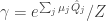
This exponential state, we argued, follows also from time evolution. The white-bean soup equilibrates upon exchanging heat and particles with the kitchen air for ages. Our quantum system can exchange observables $\hat{Q}_j$ with its environment for ages. The system equilibrates, we argued, to the state $\gamma$ . The argument relies on a quantum-information tool called canonical typicality.

Third, we defined a resource theory for thermodynamic exchanges of noncommuting observables. In a thermodynamic resource theory, the thermal states are the worthless states: From a thermal state, one can’t extract energy usable to lift a weight or to power a laptop. The worthless states, we showed, have the form of $\gamma$ .

Three path lead to the form $\gamma$ of the thermal state of a quantum system that exchanges noncommuting observables with its environment. We published the results this summer.

Not only was Team Banff spilling coffee over $\gamma$ . So were teams at Imperial College London and the University of Bristol. Our conclusions overlap, suggesting that everyone calculated correctly. Our methodologies differ, generating openings for exploration. The mountain passes between our peaks call out for mapping.

So does the path to physical reality. Do these thermal states form in labs? Could they? Cold atoms offer promise for realizations. In addition to experiments and simulations, master equations merit study. Dynamical typicality, Team Banff argued, suggests that $\gamma$ results from equilibration. Master equations model equilibration. Does some Davies-type master equation have $\gamma$ as its fixed point? Email me if you have leads!

Experimentalists, can you realize the thermal state $e^{ \sum_j \mu_j \hat{Q}_j } / Z$ whose charges $\hat{Q}_j$ don’t commute?

A photo of Banff could illustrate Merriam-Webster’s entry for “equanimity.” Banff equanimity deepened our understanding of quantum equilibrium. But we wouldn’t have understood quantum equilibrium if questions hadn’t shattered our tranquility. Give me the disequilibrium of recognizing problems, I pray, and the equilibrium to solve them.

^*By “observable,” I mean “property that you can measure.”

^**Teams at Imperial College London and Bristol asked that question, too. More pleasing than three times the coolness in Canada!

Toward a Coherent US Government Strategy for QIS

Posted on August 21, 2016 by preskill

In an upbeat recent post, Spiros reported some encouraging news about quantum information science from the US National Science and Technology Council. Today I’ll chime in with some further perspective and background.

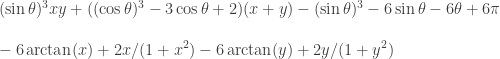
report-cover-2 The Interagency Working Group on Quantum Information Science (IWG on QIS), which began its work in late 2014, was charged “to assess Federal programs in QIS, monitor the state of the field, provide a forum for interagency coordination and collaboration, and engage in strategic planning of Federal QIS activities and investments.” The IWG recently released a well-crafted report, Advancing Quantum Information Science: National Challenges and Opportunities. The report recommends that “quantum information science be considered a priority for Federal coordination and investment.”

All the major US government agencies supporting QIS were represented on the IWG, which was co-chaired by officials from DOE, NSF, and NIST:

Steve Binkley, who heads the Advanced Scientific Computing Research (ASCR) program in the Department of Energy Office of Science,

Denise Caldwell, who directs the Physics Division of the National Science Foundation,

Carl Williams, Deputy Director of the Physical Measurement Laboratory at the National Institute for Standards and Technology.

Denise and Carl have been effective supporters of QIS over many years of government service. Steve has recently emerged as another eloquent advocate for the field’s promise and importance.

At our request, the three co-chairs fielded questions about the report, with the understanding that their responses would be broadly disseminated. Their comments reinforced the message of the report — that all cognizant agencies favor a “coherent, all-of-government approach to QIS.”

Science funding in the US differs from elsewhere in the world. QIS is a prime example — for over 20 years, various US government agencies, each with its own mission, goals, and culture, have had a stake in QIS research. By providing more options for supporting innovative ideas, the existence of diverse autonomous funding agencies can be a blessing. But it can also be bewildering for scientists seeking support, and it poses challenges for formulating and executing effective national science policy. It’s significant that many different agencies worked together in the IWG, and were able to align with a shared vision.

“I think that everybody in the group has the same goals,” Denise told us. “The nation has a tremendous opportunity here. This is a terrifically important field for all of us involved, and we all want to see it succeed.” Carl added, “All of us believe that this is an area in which the US must be competitive, it is very important for both scientific and technological reasons … The differences [among agencies] are minor.”

Asked about the timing of the IWG and its report, Carl noted the recent trend toward “emerging niche applications” of QIS such as quantum sensors, and Denise remarked that government agencies are responding to a plea from industry for a cross-disciplinary work force broadly trained in QIS. At the same time, Denise emphasized, the IWG recognizes that “there are still many open basic science questions that are important for this field, and we need to focus investment onto these basic science questions, as well as look at investments or opportunities that lead into the first applications.”

DOE’s FY2017 budget request includes $10M to fund a new QIS research program, coordinated with NIST and NSF. Steve explained the thinking behind that request: “There are problems in the physical science space, spanned by DOE Office of Science programs, where quantum computation would be a useful a tool. This is the time to start making investments in that area.” Asked about the longer term commitment of DOE to QIS research, Steve was cautious. “What it will grow into over time is hard to tell — we’re right at the beginning.”

What can the rest of us in the QIS community do to amplify the impact of the report? Carl advised: “All of us should continue getting the excitement of the field out there, [and point to] the potential long term payoffs, whether they be in searches for dark matter or building better clocks or better GPS systems or better sensors. Making everybody aware of all the potential is good for our economy, for our country, and for all of us.”

Taking an even longer view, Denise reminded us that effective advocacy for QIS can get young people “excited about a field they can work in, where they can get jobs, where they can pursue science — that can be critically important. If we all think back to our own beginning careers, at some point in time we got excited about science. And so whatever one can do to excite the next generation about science and technology, with the hope of bringing them into studying and developing careers in this field, to me this is tremendously valuable. ”

All of us in the quantum information science community owe a debt to the IWG for their hard work and eloquent report, and to the agencies they represent for their vision and support. And we are all fortunate to be participating in the early stages of a new quantum revolution. As the IWG report makes clear, the best is yet to come.

Greg Kuperberg’s calculus problem

Posted on August 3, 2016 by spiros

“How good are you at calculus?”

This was the opening sentence of Greg Kuperberg’s Facebook status on July 4th, 2016.

“I have a joint paper (on isoperimetric inequalities in differential geometry) in which we need to know that

$(\sin\theta)^3 xy + ((\cos\theta)^3 -3\cos\theta +2) (x+y) - (\sin\theta)^3-6\sin\theta -6\theta + 6\pi \\ \\- 6\arctan(x) +2x/(1+x^2) -6\arctan(y) +2y/(1+y^2)$

is non-negative for x and y non-negative and $\theta$ between $0$ and $\pi$ . Also, the minimum only occurs for $x=y=1/(\tan(\theta/2)$ .”

Let’s take a moment to appreciate the complexity of the mathematical statement above. It is a non-linear inequality in three variables, mixing trigonometry with algebra and throwing in some arc-tangents for good measure. Greg, continued:

“We proved it, but only with the aid of symbolic algebra to factor an algebraic variety into irreducible components. The human part of our proof is also not really a cake walk.

A simpler proof would be way cool.”

I was hooked. The cubic terms looked a little intimidating, but if I converted x and y into $\tan(\theta_x)$ and $\tan(\theta_y)$ , respectively, as one of the comments on Facebook promptly suggested, I could at least get rid of the annoying arc-tangents and then calculus and trigonometry would take me the rest of the way. Greg replied to my initial comment outlining a quick route to the proof: “Let me just caution that we found the problem unyielding.” Hmm… Then, Greg revealed that the paper containing the original proof was over three years old (had he been thinking about this since then? that’s what true love must be like.) Titled “The Cartan-Hadamard Conjecture and The Little Prince“, the above inequality makes its appearance as Lemma 7.1 on page 45 (of 63). To quote the paper: “Although the lemma is evident from contour plots, the authors found it surprisingly tricky to prove rigorously.”

As I filled pages of calculations and memorized every trigonometric identity known to man, I realized that Greg was right: the problem was highly intractable. The quick solution that was supposed to take me two to three days turned into two weeks of hell, until I decided to drop the original approach and stick to doing calculus with the known unknowns, x and y. The next week led me to a set of three non-linear equations mixing trigonometric functions with fourth powers of x and y, at which point I thought of giving up. I knew what I needed to do to finish the proof, but it looked freaking insane. Still, like the masochist that I am, I continued calculating away until my brain was mush. And then, yesterday, during a moment of clarity, I decided to go back to one of the three equations and rewrite it in a different way. That is when I noticed the error. I had solved for $\cos\theta$ in terms of x and y, but I had made a mistake that had cost me 10 days of intense work with no end in sight. Once I found the mistake, the whole proof came together within about an hour. At that moment, I felt a mix of happiness (duh), but also sadness, as if someone I had grown fond of no longer had a reason to spend time with me and, at the same time, I had ran out of made-up reasons to hang out with them. But, yeah, I mostly felt happiness.

Greg Kuperberg pondering about the universe of mathematics.

Before I present the proof below, I want to take a moment to say a few words about Greg, whom I consider to be the John Preskill of mathematics: a lodestar of sanity in a sea of hyperbole (to paraphrase Scott Aaronson). When I started grad school at UC Davis back in 2003, quantum information theory and quantum computing were becoming “a thing” among some of the top universities around the US. So, I went to several of the mathematics faculty in the department asking if there was a course on quantum information theory I could take. The answer was to “read Nielsen and Chuang and then go talk to Professor Kuperberg”. Being a foolish young man, I skipped the first part and went straight to Greg to ask him to teach me (and four other brave souls) quantum “stuff”. Greg obliged with a course on… quantum probability and quantum groups. Not what I had in mind. This guy was hardcore. Needless to say, the five brave souls taking the class (mostly fourth year graduate students and me, the noob) quickly became three, then two gluttons for punishment (the other masochist became one of my best friends in grad school). I could not drop the class, not because I had asked Greg to do this as a favor to me, but because I knew that I was in the presence of greatness (or maybe it was Stockholm syndrome). My goal then, as an aspiring mathematician, became to one day have a conversation with Greg where, for some brief moment, I would not sound stupid. A man of incredible intelligence, Greg is that rare individual whose character matches his intellect. Much like the anti-heroes portrayed by Humphrey Bogart in Casablanca and the Maltese Falcon, Greg keeps a low-profile, seems almost cynical at times, but in the end, he works harder than everyone else to help those in need. For example, on MathOverflow, a question and answer website for professional mathematicians around the world, Greg is listed as one of the top contributors of all time.

But, back to the problem. The past four weeks thinking about it have oscillated between phases of “this is the most fun I’ve had in years!” to “this is Greg’s way of telling me I should drop math and become a go-go dancer”. Now that the ordeal is over, I can confidently say that the problem is anything but “dull” (which is how Greg felt others on MathOverflow would perceive it, so he never posted it there). In fact, if I ever have to teach Calculus, I will subject my students to the step-by-step proof of this problem. OK, here is the proof. This one is for you Greg. Thanks for being such a great role model. Sorry I didn’t get to tell you until now. And you are right not to offer a “bounty” for the solution. The journey (more like, a trip to Mordor and back) was all the money.

The proof: The first thing to note (and if I had read Greg’s paper earlier than today, I would have known as much weeks ago) is that the following equality holds (which can be verified quickly by differentiating both sides):

$4 x - 6\arctan(x) +2x/(1+x^2) = 4 \int_0^x \frac{s^4}{(1+s^2)^2} ds$ .

Using the above equality (and the equivalent one for y), we get:

$F(\theta,x,y) = (\sin\theta)^3 xy + ((\cos\theta)^3 -3\cos\theta -2) (x+y) - (\sin\theta)^3-6\sin\theta -6\theta + 6\pi \\ \\4 \int_0^x \frac{s^4}{(1+s^2)^2} ds+4 \int_0^y \frac{s^4}{(1+s^2)^2} ds.$

Now comes the fun part. We differentiate with respect to $\theta$ , x and y, and set to zero to find all the maxima and minima of $F(\theta,x,y)$ (though we are only interested in the global minimum, which is supposed to be at $x=y=\tan^{-1}(\theta/2))$ . Some high-school level calculus yields:

$\partial_\theta F(\theta,x,y) = 0 \implies \sin^2(\theta) (\cos(\theta) xy + \sin(\theta)(x+y)) = \\ \\ 2 (1+\cos(\theta))+\sin^2(\theta)\cos(\theta).$

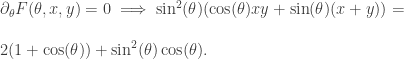
At this point, the most well-known trigonometric identity of all time, $\sin^2(\theta)+\cos^2(\theta)=1$ , can be used to show that the right-hand-side can be re-written as:

$2(1+\cos(\theta))+\sin^2(\theta)\cos(\theta) = \sin^2(\theta) (\cos\theta \tan^{-2}(\theta/2) + 2\sin\theta \tan^{-1}(\theta/2)),$

where I used (my now favorite) trigonometric identity: $\tan^{-1}(\theta/2) = (1+\cos\theta)/\sin(\theta)$ (note to the reader: $\tan^{-1}(\theta) = \cot(\theta)$ ). Putting it all together, we now have the very suggestive condition:

$\sin^2(\theta) (\cos(\theta) (xy-\tan^{-2}(\theta/2)) + \sin(\theta)(x+y-2\tan^{-1}(\theta/2))) = 0,$

noting that, despite appearances, $\theta = 0$ is not a solution (as can be checked from the original form of this equality, unless $x$ and $y$ are infinite, in which case the expression is clearly non-negative, as we show towards the end of this post). This leaves us with $\theta = \pi$ and

$\cos(\theta) (\tan^{-2}(\theta/2)-xy) = \sin(\theta)(x+y-2\tan^{-1}(\theta/2)),$

as candidates for where the minimum may be. A quick check shows that:

$F(\pi,x,y) = 4 \int_0^x \frac{s^4}{(1+s^2)^2} ds+4 \int_0^y \frac{s^4}{(1+s^2)^2} ds \ge 0,$

since x and y are non-negative. The following obvious substitution becomes our greatest ally for the rest of the proof:

$x= \alpha \tan^{-1}(\theta/2), \, y = \beta \tan^{-1}(\theta/2).$

Substituting the above in the remaining condition for $\partial_\theta F(\theta,x,y) = 0$ , and using again that $\tan^{-1}(\theta/2) = (1+\cos\theta)/\sin\theta$ , we get:

$\cos\theta (1-\alpha\beta) = (1-\cos\theta) ((\alpha-1) + (\beta-1)),$

which can be further simplified to (if you are paying attention to minus signs and don’t waste a week on a wild-goose chase like I did):

$\cos\theta = \frac{1}{1-\beta}+\frac{1}{1-\alpha}$ .

As Greg loves to say, we are finally cooking with gas. Note that the expression is symmetric in $\alpha$ and $\beta$ , which should be obvious from the symmetry of $F(\theta,x,y)$ in x and y. That observation will come in handy when we take derivatives with respect to x and y now. Factoring $(\cos\theta)^3 -3\cos\theta -2 = - (1+\cos\theta)^2(2-\cos\theta)$ , we get:

$\partial_x F(\theta,x,y) = 0 \implies \sin^3(\theta) y + 4\frac{x^4}{(1+x^2)^2} = (1+\cos\theta)^2 + \sin^2\theta (1+\cos\theta).$

Substituting x and y with $\alpha \tan^{-1}(\theta/2), \beta \tan^{-1}(\theta/2)$ , respectively and using the identities $\tan^{-1}(\theta/2) = (1+\cos\theta)/\sin\theta$ and $\tan^{-2}(\theta/2) = (1+\cos\theta)/(1-\cos\theta),$ the above expression simplifies significantly to the following expression:

$4\alpha^4 =\left((\alpha^2-1)\cos\theta+\alpha^2+1\right)^2 \left(1 + (1-\beta)(1-\cos\theta)\right).$

Using $\cos\theta = \frac{1}{1-\beta}+\frac{1}{1-\alpha}$ , which we derived earlier by looking at the extrema of $F(\theta,x,y)$ with respect to $\theta$ , and noting that the global minimum would have to be an extremum with respect to all three variables, we get:

$4\alpha^4 (1-\beta) = \alpha (\alpha-1) (1+\alpha + \alpha(1-\beta))^2,$

where we used $1 + (1-\beta)(1-\cos\theta) = \alpha (1-\beta) (\alpha-1)^{-1}$ and

$(\alpha^2-1)\cos\theta+\alpha^2+1 = (\alpha+1)((\alpha-1)\cos\theta+1)+\alpha(\alpha-1) = \\ (\alpha-1)(1-\beta)^{-1} (2\alpha + 1-\alpha\beta).$

We may assume, without loss of generality, that $x \ge y$ . If $\alpha = 0$ , then $\alpha = \beta = 0$ , which leads to the contradiction $\cos\theta = 2$ , unless the other condition, $\theta = \pi$ , holds, which leads to $F(\pi,0,0) = 0$ . Dividing through by $\alpha$ and re-writing $4\alpha^3(1-\beta) = 4\alpha(1+\alpha)(\alpha-1)(1-\beta) + 4\alpha(1-\beta)$ , yields:

$4\alpha (1-\beta) = (\alpha-1) (1+\alpha - \alpha(1-\beta))^2 = (\alpha-1)(1+\alpha\beta)^2,$

which can be further modified to:

$4\alpha +(1-\alpha\beta)^2 = \alpha (1+\alpha\beta)^2,$

and, similarly for $\beta$ (due to symmetry):

$4\beta +(1-\alpha\beta)^2 = \beta (1+\alpha\beta)^2.$

Subtracting the two equations from each other, we get:

$4(\alpha-\beta) = (\alpha-\beta)(1+\alpha\beta)^2$ ,

which implies that $\alpha = \beta$ and/or $\alpha\beta =1$ . The first leads to $4\alpha (1-\alpha) = (\alpha-1)(1+\alpha^2)^2,$ which immediately implies $\alpha = 1 = \beta$ (since the left and right side of the equality have opposite signs otherwise). The second one implies that either $\alpha+\beta =2$ , or $\cos\theta =1$ , which follows from the earlier equation $\cos\theta (1-\alpha\beta) = (1-\cos\theta) ((\alpha-1) + (\beta-1))$ . If $\alpha+\beta =2$ and $1 = \alpha\beta$ , it is easy to see that $\alpha=\beta=1$ is the only solution by expanding $(\sqrt{\alpha}-\sqrt{\beta})^2=0$ . If, on the other hand, $\cos\theta = 1$ , then looking at the original form of $F(\theta,x,y)$ , we see that $F(0,x,y) = 6\pi - 6\arctan(x) +2x/(1+x^2) -6\arctan(y) +2y/(1+y^2) \ge 0$ , since $x,y \ge 0 \implies \arctan(x)+\arctan(y) \le \pi$ .

And that concludes the proof, since the only cases for which all three conditions are met lead to $\alpha = \beta = 1$ and, hence, $x=y=\tan^{-1}(\theta/2)$ . The minimum of $F(\theta, x,y)$ at these values is always zero. That’s right, all this work to end up with “nothing”. But, at least, the last four weeks have been anything but dull.

Update: Greg offered Lemma 7.4 from the same paper as another challenge (the sines, cosines and tangents are now transformed into hyperbolic trigonometric functions, with a few other changes, mostly in signs, thrown in there). This is a more hardcore-looking inequality, but the proof turns out to follow the steps of Lemma 7.1 almost identically. In particular, all the conditions for extrema are exactly the same, with the only difference being that cosine becomes hyperbolic cosine. It is an awesome exercise in calculus to check this for yourself. Do it. Unless you have something better to do.

Quantum Supremacy: The US gets serious

Posted on July 31, 2016 by spiros

If you have been paying any attention to the news on quantum computing and the evolution of industrial and national efforts towards realizing a scalable, fault-tolerant quantum computer that can tackle problems intractable to current supercomputing capabilities, then you know that something big is stirring throughout the quantum world.

More than 15 years ago, Microsoft decided to jump into the quantum computing business betting big on topological quantum computing as the next big thing. The new website of Microsoft’s Station Q shows that keeping a low profile is no longer an option. This is a sentiment that Google clearly shared, when back in 2013, they decided to promote their new partnership with NASA Ames and D-Wave, known as the Quantum A.I. Lab, through a YouTube video that went viral (disclosure: they do own Youtube.) In fact, IQIM worked with Google at the time to get kids excited about the quantum world by developing qCraft, a mod introducing quantum physics into the world of Minecraft. Then, a few months ago, IBM unveiled the quantum experience website, which captured the public’s imagination by offering a do-it-yourself opportunity to run an algorithm on a 5-qubit quantum chip in the cloud.

But, looking at the opportunities for investment in academic groups working on quantum computing, companies like Microsoft were/are investing heavily in experimental labs across the pond, such as Leo Kowenhoven’s group at TU Delft and Charlie Marcus’ group in Copenhagen, with smaller investments here in the US. This may just reflect the fact that the best efforts to build topological qubits are in Europe, but it still begs the question why a fantastic idea like topologically protected majorana zero modes, by Yale University’s Nick Read and Dmitry Green, which inspired the now famous Majorana wire paper by Alexei Kitaev when he was a researcher at Microsoft’s Redmond research lab, and whose transition from theory to experiment took off with contributions from Maryland and IQIM researchers, was outsourced to European labs for experimental verification and further development. The one example of a large investment in a US academic research group has been Google’s hiring of John Martinis away from UCSB. In fact, John and I met a couple of years ago to discuss investment into his superconducting quantum computing efforts, because government funding for academic efforts to actually build a quantum computer was lacking. China was investing, Canada was investing, Europe went a little crazy, but the US was relying on visionary agencies like IARPA, DARPA and the NSF to foot the bill (without which Physics Frontiers Centers like IQIM wouldn’t be around). In short, there was no top-down policy directive to focus national attention and inter-agency Federal funding on winning the quantum supremacy race.

Until now.

The National Science and Technology Council, which is chaired by the President of the United States and “is the principal means within the executive branch to coordinate science and technology policy across the diverse entities that make up the Federal research and development enterprise”, just released the following report:

Advancing Quantum Information Science: National Challenges and Opportunities

The White House blog post does a good job at describing the high-level view of what the report is about and what the policy recommendations are. There is mention of quantum sensors and metrology, of the promise of quantum computing to material science and basic science, and they even go into the exciting connections between quantum error-correcting codes and emergent spacetime, by IQIM’s Pastawski, et al.

But the big news is that the report recommends significant and sustained investment in Quantum Information Science. The blog post reports that the administration intends “to engage academia, industry, and government in the upcoming months to … exchange views on key needs and opportunities, and consider how to maintain vibrant and robust national ecosystems for QIS research and development and for high-performance computing.”

Personally, I am excited to see how the fierce competition at the academic, industrial and now international level will lead to a race for quantum supremacy. The rivals are all worthy of respect, especially because they are vying for supremacy not just over each other, but over a problem so big and so interesting, that anyone’s success is everyone’s success. After all, anyone can quantum, and if things go according to plan, we will soon have the first generation of kids trained on hourofquantum.com (it doesn’t exist yet), as well as hourofcode.com. Until then, quantum chess and qCraft will have to do.

Bringing the heat to Cal State LA

Posted on July 24, 2016 by Nicole Yunger Halpern

John Baez is a tough act to follow.

The mathematical physicist presented a colloquium at Cal State LA this May.¹ The talk’s title: “My Favorite Number.” The advertisement image: A purple “24” superimposed atop two egg cartons.

The colloquium concerned string theory. String theorists attempt to reconcile Einstein’s general relativity with quantum mechanics. Relativity concerns the large and the fast, like the sun and light. Quantum mechanics concerns the small, like atoms. Relativity and with quantum mechanics individually suggest that space-time consists of four dimensions: up-down, left-right, forward-backward, and time. String theory suggests that space-time has more than four dimensions. Counting dimensions leads theorists to John Baez’s favorite number.

His topic struck me as bold, simple, and deep. As an otherworldly window onto the pedestrian. John Baez became, when I saw the colloquium ad, a hero of mine.

And a tough act to follow.

I presented Cal State LA’s physics colloquium the week after John Baez. My title: “Quantum steampunk: Quantum information applied to thermodynamics.” Steampunk is a literary, artistic, and film genre. Stories take place during the 1800s—the Victorian era; the Industrial era; an age of soot, grime, innovation, and adventure. Into the 1800s, steampunkers transplant modern and beyond-modern technologies: automata, airships, time machines, etc. Example steampunk works include Will Smith’s 1999 film Wild Wild West. Steampunk weds the new with the old.

So does quantum information applied to thermodynamics. Thermodynamics budded off from the Industrial Revolution: The steam engine crowned industrial technology. Thinkers wondered how efficiently engines could run. Thinkers continue to wonder. But the steam engine no longer crowns technology; quantum physics (with other discoveries) does. Quantum information scientists study the roles of information, measurement, and correlations in heat, energy, entropy, and time. We wed the new with the old.

What image could encapsulate my talk? I couldn’t lean on egg cartons. I proposed a steampunk warrior—cravatted, begoggled, and spouting electricity. The proposal met with a polite cough of an email. Not all department members, Milan Mijic pointed out, had heard of steampunk.

Milan is a Cal State LA professor and my erstwhile host. We toured the palm-speckled campus around colloquium time. What, he asked, can quantum information contribute to thermodynamics?

Heat offers an example. Imagine a classical (nonquantum) system of particles. The particles carry kinetic energy, or energy of motion: They jiggle. Particles that bump into each other can exchange energy. We call that energy heat. Heat vexes engineers, breaking transistors and lowering engines’ efficiencies.

Like heat, work consists of energy. Work has more “orderliness” than the heat transferred by random jiggles. Examples of work exertion include the compression of a gas: A piston forces the particles to move in one direction, in concert. Consider, as another example, driving electrons around a circuit with an electric field. The field forces the electrons to move in the same direction. Work and heat account for all the changes in a system’s energy. So states the First Law of Thermodynamics.

Suppose that the system is quantum. It doesn’t necessarily have a well-defined energy. But we can stick the system in an electric field, and the system can exchange motional-type energy with other systems. How should we define “work” and “heat”?

Quantum information offers insights, such as via entropies. Entropies quantify how “mixed” or “disordered” states are. Disorder grows as heat suffuses a system. Entropies help us extend the First Law to quantum theory.

So I explained during the colloquium. Rarely have I relished engaging with an audience as much as I relished engaging with Cal State LA’s. Attendees made eye contact, posed questions, commented after the talk, and wrote notes. A student in a corner appeared to be writing homework solutions. But a presenter couldn’t have asked for more from the rest. One exclamation arrested me like a coin in the cogs of a grandfather clock.

I’d peppered my slides with steampunk art: paintings, drawings, stills from movies. The peppering had staved off boredom as I’d created the talk. I hoped that the peppering would stave off my audience’s boredom. I apologized about the trimmings.

“No!” cried a woman near the front. “It’s lovely!”

I was about to discuss experiments by Jukka Pekola’s group. Pekola’s group probes quantum thermodynamics using electronic circuits. The group measures heat by counting the electrons that hop from one part of the circuit to another. Single-electron transistors track tunneling (quantum movements) of single particles.

Heat complicates engineering, calculations, and California living. Heat scrambles signals, breaks devices, and lowers efficiencies. Quantum heat can evade definition. Thermodynamicists grind their teeth over heat.

“No!” the woman near the front had cried. “It’s lovely!”

She was referring to steampunk art. But her exclamation applied to my subject. Heat has not only practical importance, but also fundamental: Heat influences every law of thermodynamics. Thermodynamic law underpins much of physics as 24 underpins much of string theory. Lovely, I thought, indeed.

Cal State LA offered a new view of my subfield, an otherworldly window onto the pedestrian. The more pedestrian an idea—the more often the idea surfaces, the more of our world the idea accounts for—the deeper the physics. Heat seems as pedestrian as a Pokémon Go player. But maybe, someday, I’ll present an idea as simple, bold, and deep as the number 24.

A window onto Cal State LA.

With gratitude to Milan Mijic, and to Cal State LA’s Department of Physics and Astronomy, for their hospitality.

¹For nonacademics: A typical physics department hosts several presentations per week. A seminar relates research that the speaker has undertaken. The audience consists of department members who specialize in the speaker’s subfield. A department’s astrophysicists might host a Monday seminar; its quantum theorists, a Wednesday seminar; etc. One colloquium happens per week. Listeners gather from across the department. The speaker introduces a subfield, like the correction of errors made by quantum computers. Course lectures target students. Endowed lectures, often named after donors, target researchers.

The physics of Trump?? Election renormalization.

Image

Two things were high in my mind this last quarter: My course on advanced statistical mechanics and phase transitions, and the bizarre general elections that raged all around. It is no wonder then, that I would start to conflate the Ising model, Landau mean field, and renormalization group, with the election process, and just think of each and every one of us as a tiny magnet, that needs to say up or down – Trump or Cruz, Clinton or Sanders (a more appetizing choice, somehow), and .. you get the drift.

Elections and magnetic phase transitions are very much alike. The latter, I will argue, teaches us something very important about the former.

The physics of magnetic phase transitions is amazing. If I hadn’t thought this way, I wouldn’t be a condensed matter physicist. Models of magnets consider a bunch of spins – each one a small magnet – that talk only to their nearest neighbor, as happens in typical magnets. At the onset of magnetic order (the Curie temperature), when the symmetry of the spins becomes broken, it turns out that the spin correlation length diverges. Even though Interaction length = lattice constant, we get correlation length = infinity.

To understand how ridiculous this is, you should understand what a correlation length is. The correlation tells you a simple thing. If you are a spin, trying to make it out in life, and trying to figure out where to point, your pals around you are certainly going to influence you. Their pals will influence them, and therefore you. The correlation length tells you how distant can a spin be, and still manage to nudge you to point up or down. In physics-speak, it is the reduced correlation length. It makes sense that somebody in you neighborhood, or your office, or even your town, will do something that will affect you – after all – you always interact with people that distant. But the analogy to the spins is that there is always a given circumstance where some random person in Incheon, South Korea, could influence your vote. A diverging correlation length is the Butterfly effect for real.

And yet, spins do this. At the critical temperature, just as the spins decide whether they want to point along the north pole or towards Venus, every nonsense of a fluctuation that one of them makes leagues away may galvanize things one way or another. Without ever even remotely directly talking to even their father’s brother’s nephew’s cousin’s former roommate! Every fluctuation, no matter where, factors into the symmetry breaking process.

A bit of physics, before I’m blamed for being crude in my interpretation. The correlation length at the Curie point, and almost all symmetry-breaking continuous transitions, diverges as some inverse power of the temperature difference to the critical point: $\frac{1}{|T-T_c|}^{\nu}$ . The faster it diverges (the higher the power $\nu$ ) , actually the more feeble the symmetry breaking is. Why is that? After I argued that this is an amazing phenomenon? Well, if $10^2$ voices can shift you one way or another, each voice is worth something. If $10^{20}$ voices are able to push you around, I’m not really buying influence on you by bribing ten of these. Each voice is worth less. Why? The correlation length is also a measure of the uncertainty before the moment of truth – when the battle starts and we don’t know who wins. Big correlation length – any little element of the battlefield can change something, and many souls are involved and active. Small correlation length – the battle was already decided since one of the sides has a single bomb that will evaporate the world. Who knew that Dr. Strangelove could be a condensed matter physicist?

This lore of correlations led to one of the most breathtaking developments of 20^th century physics. I’m a condensed matter guy, so it is natural that Ken Wilson, as well as Ben Widom, Michael Fisher, and Leo Kadanoff are my superheros. They came up with an idea so simple yet profound – scaling. If you have a system (say, of spins) that you can’t figure out – maybe because it is fluctuating, and because it is interacting – regardless, all you need to do is to move away from it. Let averaging (aka, central limit theorem) do the job and suppress fluctuations. Let us just zoom out. If we change the scale by a factor of 2, so that all spins look more crowded, then the correlation length also look half as big. The system looks less critical. It is as if we managed to move away from the critical temperature – either cooling towards $T=0$ , or heating up towards $T=\infty$ . Both limits are easy to solve. How do we make this into a framework? If the pre-zoom-out volume had 8 spins, we can average them into a representative single spin. This way you’ll end up with a system that looks pretty much like the one you had before – same spin density, same interaction, same physics – but at a different temperature, and further from the phase transition. It turns out you can do this, and you can figure out how much changed in the process. Together, this tells you how the correlation length depends on $T-T_c$ . This is the renormalization group, aka, RG.

Interestingly, this RG procedure informs us that criticality and symmetry breaking are more feeble the lower the dimension. There are no 1d permanent magnets, and magnetism in 2d is very frail. Why? Well, the more dimensions there are, the more nearest neighbors each spin has, and more neighbors your neighbors have. Think about the 6-degrees of separation game. 3d is okay for magnets, as we know. It turns out, however, that in physical systems above 4 dimensions, critical phenomena is the same as that of a fully connected (infinite dimensional) network. The uncertainty stage is very small, correlations length diverge slowly. Even at distance 1 there are enough people or spins to bend your will one way or another. Magnetization is just a question of time elapsed from the beginning of the experiment.

Spins, votes, what’s the difference? You won’t be surprised to find that the term renormalization has permeated every aspect of economics and social science as well. What is voting Republican vs Democrat if not a symmetry breaking? Well, it is not that bad yet – the parties are different. No real symmetry there, you would think. Unless you ask the ‘undecided voter’.

And if elections are affected by such correlated dynamics, what about revolutions? Here the analogy with phase transitions is so much more prevalent even in our language – resistance to a regime solidifies, crystallizes, and aligns – just like solids and magnets. When people are fed up with a regime, the crucial question is – if I would go to the streets, will I be joined by enough people to affect a change?

Revolutions, therefore, seem to rise out of strong fluctuations in the populace. If you wish, think of revolutions as domains where the frustration is so high, which give a political movement the inertia it needs.

Domains-: that’s exactly what the correlation length is about. The correlation length is the size of correlated magnetic domains, i.e.,groups of spins that point in the same direction. And now we remember that close to a phase transition, the correlation length diverges as some power of the distance ot the transition: $\frac{1}{|T-T_c|^{\nu}}$ . Take a magnet just above its Curie temperature. The closer we are to a phase transition, the larger the correlation length is, and the bigger are the fluctuating magnetized domains. The parameter $\nu$ is the correlation-length critical exponent and something of a holy grail for practitioners of statistical mechanics. Everyone wants to calculate it for various phase transition. It is not that easy. That’s partially why I have a job.

The correlation length aside, how many spins are involved in a domain? $\left[1/|T-T_c|^d\right]^{\nu}$ . Actually, we know roughly what $\nu$ is. For systems with dimension $latex d>4$, it is ½. For systems with a lower dimensionality it is roughly $latex 2/d$. (Comment for the experts: I’m really not kidding – this fits the Ising model for 2 and 3 dimensions, and it fits the xy model for 3d).

So the number of spins in a domain in systems below 4d is $1/|T-T_c|^2$ , independent of dimension. On the other hand, four d and up it is $1/|T-T_c|^{d/2}$ . Increasing rapidly with dimension, when we are close to the critical point.

Back to voters. In a climate of undecided elections, analogous to a magnet near its Curie point, the spins are the voters, and domain walls are the crowds supporting this candidate or that policy; domain walls are what becomes large demonstrations in the Washington Mall. And you would think that the world we live in is clearly 2d – a surface of a 3d sphere (and yes – that includes Manhattan!). So a political domain size just diverges as a simple moderate $1/|T-T_c|^2$ during times of contested elections.

Something happened, however, in the past two decades: the internet. The connectivity of the world has changed dramatically.

No more 2d. Now, our effective dimension is determined by our web based social network. Facebook perhaps? Roughly speaking, the dimensionality of the Facebook network is that number of friends we have, divided by the number of mutual friends. I venture to say this averages at about 10. With about a 150 friends in tow, out of which 15 are mutual. So our world, for election purposes, is 10 dimensional big!

Let’s simulate what this means for our political system. Any event – a terrorist attack, or a recession, etc. will cause a fluctuation that will involve a large group of people – a domain. Take a time when $T-T_c$ is a healthy $0.1$ for instance. In the good old $2d$ world this would involve 100 friends times $1/0.1^2\sim 10000$ people. Now it would be more like $100\cdot 1/0.1^{10/2}\sim 10$ -millions. So any small perturbation of conditions could make entire states turn one way or another.

When response to slight shifts in prevailing conditions encompasses entire states, rather than entire neighborhoods, polarization follows. Over all, a state where each neighborhood has a slightly different opinion will be rather moderate – extreme opinions will only resonate locally. Single voices could only sway so many people. But nowadays, well – we’ve all seen Trump and the like on the march. Millions. It’s not even their fault – its physics!

Can we do anything about it? It’s up for debate. Maybe cancel the electoral college, to make the selecting unit larger than the typical size of a fluctuating domain. Maybe carry out a time averaged election: make an election year where each month there is a contest for the grand prize. Or maybe just move to Canada.

What matters to me, and why?

Posted on June 26, 2016 by Nicole Yunger Halpern

Students at my college asked every Tuesday. They gathered in a white, windowed room near the center of campus. “We serve,” read advertisements, “soup, bread, and food for thought.” One professor or visitor would discuss human rights, family, religion, or another pepper in the chili of life.

I joined occasionally. I listened by the window, in the circle of chairs that ringed the speaker. Then I ventured from college into physics.

The questions “What matters to you, and why?” have chased me through physics. I ask experimentalists and theorists, professors and students: Why do you do science? Which papers catch your eye? Why have you devoted to quantum information more years than many spouses devote to marriages?

One physicist answered with another question. Chris Jarzynski works as a professor at the University of Maryland. He studies statistical mechanics—how particles typically act and how often particles act atypically; how materials shine, how gases push back when we compress them, and more.

“How,” Chris asked, “should we quantify precision?”

Chris had in mind nonequilibrium fluctuation theorems. Out-of-equilibrium systems have large-scale properties, like temperature, that change significantly.¹ Examples include white-bean soup cooling at a “What matters” lunch. The soup’s temperature drops to room temperature as the system approaches equilibrium.

Nonequilibrium. Tasty, tasty nonequilibrium.

Some out-of-equilibrium systems obey fluctuation theorems. Fluctuation theorems are equations derived in statistical mechanics. Imagine a DNA molecule floating in a watery solution. Water molecules buffet the strand, which twitches. But the strand’s shape doesn’t change much. The DNA is in equilibrium.

You can grab the strand’s ends and stretch them apart. The strand will leave equilibrium as its length changes. Imagine pulling the strand to some predetermined length. You’ll have exerted energy.

How much? The amount will vary if you repeat the experiment. Why? This trial began with the DNA curled this way; that trial began with the DNA curled that way. During this trial, the water batters the molecule more; during that trial, less. These discrepancies block us from predicting how much energy you’ll exert. But suppose you pick a number W. We can form predictions about the probability that you’ll have to exert an amount W of energy.

How do we predict? Using nonequilibrium fluctuation theorems.

Fluctuation theorems matter to me, as Quantum Frontiers regulars know. Why? Because I’ve written enough fluctuation-theorem articles to test even a statistical mechanic’s patience. More seriously, why do fluctuation theorems matter to me?

Fluctuation theorems fill a gap in the theory of statistical mechanics. Fluctuation theorems relate nonequilibrium processes (like the cooling of soup) to equilibrium systems (like room-temperature soup). Physicists can model equilibrium. But we know little about nonequilibrium. Fluctuation theorems bridge from the known (equilibrium) to the unknown (nonequilibrium).

Experiments take place out of equilibrium. (Stretching a DNA molecule changes the molecule’s length.) So we can measure properties of nonequilibrium processes. We can’t directly measure properties of equilibrium processes, which we can’t perform experimentally. But we can measure an equilibrium property indirectly: We perform nonequilibrium experiments, then plug our data into fluctuation theorems.

Which equilibrium property can we infer about? A free-energy difference, denoted by ΔF. Every equilibrated system (every room-temperature soup) has a free energy F. F represents the energy that the system can exert, such as the energy available to stretch a DNA molecule. Imagine subtracting one system’s free energy, F₁, from another system’s free energy, F₂. The subtraction yields a free-energy difference, ΔF = F₂ – F₁. We can infer the value of a ΔF from experiments.

How should we evaluate those experiments? Which experiments can we trust, and which need repeating?

Those questions mattered little to me, before I met Chris Jarzynski. Bridging equilibrium with nonequilibrium mattered to me, and bridging theory with experiment. Not experimental nitty-gritty.

I deserved a dunking in white-bean soup.

Suppose you performed infinitely many trials—stretched a DNA molecule infinitely many times. In each trial, you measured the energy exerted. You processed your data, then substituted into a fluctuation theorem. You could infer the exact value of ΔF.

But we can’t perform infinitely many trials. Imprecision mars our inference about ΔF. How does the imprecision relate to the number of trials performed?²

Chris and I adopted an information-theoretic approach. We quantified precision with a parameter $\delta$ . Suppose you want to estimate ΔF with some precision. How many trials should you expect to need to perform? We bounded the number $N_\delta$ of trials, using an entropy. The bound tightens an earlier estimate of Chris’s. If you perform $N_\delta$ trials, you can estimate ΔF with a percent error that we estimated. We illustrated our results by modeling a gas.

I’d never appreciated the texture and richness of precision. But richness precision has: A few decimal places distinguish Albert Einstein’s general theory of relativity from Isaac Newton’s 17th-century mechanics. Particle physicists calculate constants of nature to many decimal places. Such a calculation earned a nod on physicist Julian Schwinger’s headstone. Precision serves as the bread and soup of much physics. I’d sniffed the importance of precision, but not tasted it, until questioned by Chris Jarzynski.

The questioning continues. My college has discontinued its “What matters” series. But I ask scientist after scientist—thoughtful human being after thoughtful human being—“What matters to you, and why?” Asking, listening, reading, calculating, and self-regulating sharpen my answers those questions. My answers often squish beneath the bread knife in my cutlery drawer of criticism. Thank goodness that repeating trials can reduce our errors.

¹Or large-scale properties that will change. Imagine connecting the ends of a charged battery with a wire. Charge will flow from terminal to terminal, producing a current. You can measure, every minute, how quickly charge is flowing: You can measure how much current is flowing. The current won’t change much, for a while. But the current will die off as the battery nears depletion. A large-scale property (the current) appears constant but will change. Such a capacity to change characterizes nonequilibrium steady states (NESSes). NESSes form our second example of nonequilibrium states. Many-body localization forms a third, quantum example.

²Readers might object that scientists have tools for quantifying imprecision. Why not apply those tools? Because ΔF equals a logarithm, which is nonlinear. Other authors’ proposals appear in references 1-13 of our paper. Charlie Bennett addressed a related problem with his “acceptance ratio.” (Bennett also blogged about evil on Quantum Frontiers last month.)

Schopenhauer and the Geometry of Evil

Posted on May 29, 2016 by Charles H. Bennett

Gottfried_Wilhelm_von_Leibniz At the beginning of the 18th century, Gottfried Leibniz took a break from quarreling with Isaac Newton over which of them had invented calculus to confront a more formidable adversary, Evil. His landmark 1710 book Théodicée argued that, as creatures of an omnipotent and benevolent God, we live in the best of all possible worlds. Earthquakes and wars, he said, are compatible with God’s benevolence because they may lead to beneficial consequences in ways we don’t understand. Moreover, for us as individuals, having the freedom to make bad decisions challenges us to learn from our mistakes and improve our moral characters.

In 1844 another philosopher, Arthur Schopenhauer, came to the opposite conclusion,

that we live in the worst of all possible worlds. By this he meant not just a world is full of calamity and suffering, but one that in many respects, both human and natural, functions so badly that if it were only a little worse it could not continue to exist at all. An atheist, Schopenhauer felt no need to defend God’s benevolence, and could turn his full attention to the mechanics and indeed (though not a mathematician) the geometry of badness. He argued that if the world’s continued existence depends on many continuous variables such as temperature, composition of the atmosphere, etc., each of which must be within a narrow range, then almost all possible worlds will be just barely possible, lying near the periphery of the possible region. Here, in his own words, is his refutation of Leibniz’ optimism.

To return, then to Leibniz, I cannot ascribe to the Théodicée as a methodical and broad unfolding of optimism, any other merit than this, that it gave occasion later for the immortal “Candide” of the great Voltaire; whereby certainly Leibniz s often-repeated and lame excuse for the evil of the world, that the bad sometimes brings about the good, received a confirmation which was unexpected by him… But indeed to the palpably sophistical proofs of Leibniz that this is the best of all possible worlds, we may seriously and honestly oppose the proof that it is the worst of all possible worlds. For possible means, not what one may construct in imagination, but what can actually exist and continue. Now this world is so arranged as to be able to maintain itself with great difficulty; but if it were a little worse, it could no longer maintain itself. Consequently a worse world, since it could not continue to exist, is absolutely impossible: thus this world itself is the worst of all possible worlds. For not only if the planets were to run their heads together, but even if any one of the actually appearing perturbations of their course, instead of being gradually balanced by others, continued to increase, the world would soon reach its end. Astronomers know upon what accidental circumstances principally the irrational relation to each other of the periods of revolution this depends, and have carefully calculated that it will always go on well; consequently the world also can continue and go on. We will hope that, although Newton was of an opposite opinion, they have not miscalculated, and consequently that the mechanical perpetual motion realised in such a planetary system will not also, like the rest, ultimately come to a standstill. Again, under the firm crust of the planet dwell the powerful forces of nature which, as soon as some accident affords them free play, must necessarily destroy that crust, with everything living upon it, as has already taken place at least three times upon our planet, and will probably take place oftener still. The earthquake of Lisbon, the earthquake of Haiti, the destruction of Pompeii, are only small, playful hints of what is possible. A small alteration of the atmosphere, which cannot even be chemically proved, causes cholera, yellow fever, black death, &c., which carry off millions of men; a somewhat greater alteration would extinguish all life. A very moderate increase of heat would dry up all the rivers and springs. The brutes have received just barely so much in the way of organs and powers as enables them to procure with the greatest exertion sustenance for their own lives and food for their offspring; therefore if a brute loses a limb, or even the full use of one, it must generally perish. Even of the human race, powerful as are the weapons it possesses in understanding and reason, nine-tenths live in constant conflict with want, always balancing themselves with difficulty and effort upon the brink of destruction. Thus throughout, as for the continuance of the whole, so also for that of each individual being the conditions are barely and scantily given, but nothing over. The individual life is a ceaseless battle for existence itself; while at every step destruction threatens it. Just because this threat is so often fulfilled provision had to be made, by means of the enormous excess of the germs, that the destruction of the individuals should not involve that of the species, for which alone nature really cares. The world is therefore as bad as it possibly can be if it is to continue to be at all. Q. E. D. The fossils of the entirely different kinds of animal species which formerly inhabited the planet afford us, as a proof of our calculation, the records of worlds the continuance of which was no longer possible, and which consequently were somewhat worse than the worst of possible worlds.*

Writing at a time when diseases were thought to be caused by poisonous vapors, and when “germ” meant not a pathogen but a seed or embryo, Schopenhauer hints at Darwin and Wallace’s natural selection. But more importantly, as Alejandro Jenkins pointed out, Schopenhauer’s distinction between possible and impossible worlds may be the first adequate statement of what in the 20th century came to be called the weak anthropic principle, the thesis that our perspective on the universe is unavoidably biased toward conditions hospitable to the existence and maintenance of complex structures. His examples of orbital instability and lethal atmospheric changes show that by an “impossible” world he meant one that might continue to exist physically, but would extinguish beings able to witness its existence.

In Schopenhauer’s time only seven planets were known, so, given all the ways things might go wrong, and barring divine assistance, it would have required incredible good luck for even one of them to be habitable. Thus Schopenhauer’s principle, as it might better be called, was less satisfactory as an answer to the problem of existence than to the problem of evil. The belief that such extreme good luck is less plausible than deliberate creation by some sort of intelligent agent, encapsulated by Schopenhauer’s contemporary William Paley in his watchmaker analogy, remains popular today, but its cogency has been greatly diminished by two centuries of progress in astronomy. In place of Schopenhauer’s seven, the universe is now believed to contain about as many planets as there are atoms in a pencil. And that’s just the observable part, within a Hubble distance of the earth; inflationary cosmology implies that there are many more beyond our cosmological horizon, perhaps infinitely many. In such a vast universe, it is no longer surprising that some places should be habitable. In this setting Schopenhauer’s principle leads to a situation that is locally precarious but globally stable, lying between Leibniz’ unrealistic optimum and what would be a true pessimum, a globally dead universe with no life, civilization, etc. anywhere. To paraphrase Schopenhauer, modern astronomy has revealed an enormous excess of habitable places, mostly just barely habitable, so that the extinction of life in one does not entail extinction of life in the universe, for which alone nature really cares.

Returning to Schopenhauer’s refutation of Leibniz’s optimism, his qualitative verbal reasoning can easily be recast in terms of high-dimensional geometry. Let the goodness g of a possible world X be approximated to lowest order as

g(X) = 1-q(X),

where q is a positive definite quadratic form in the d-dimensional real variable X. Possible worlds correspond to X values where g is positive, lying under a paraboloidal cap centered on the optimum, g(0)=1, with negative values of g representing impossible worlds. Leaving out the impossible worlds, simple integration, of the sort Leibniz invented, shows that the average of g over possible worlds is 1-d/(d+2). So if there is one variable, the average world is 2/3 as good as the best possible, while if there are 198 variables the average world is only 1% as good. Thus, in the limit of many dimensions, the average world approaches g=0, the worst possible. More general versions of this idea can be developed using post-18’th century mathematical tools like Lipschitz continuity.

Earthquakes are an oft-cited example of senseless evil, hard to fit into a beneficent divine plan, but today we understand them as impersonal consequences of slow convection in the Earth’s mantle, which in turn is driven by the heat of its molten iron core. Another consequence of the Earth’s molten core is its magnetic field, which deflects solar wind particles and keeps them from blowing away our atmosphere. Lacking this protection, Mars lost most of its formerly dense atmosphere long ago.

One of my adult children, a surgeon, went to Haiti in 2010 to treat victims of the great earthquake and has returned regularly since. Opiate painkillers, he says, are in short supply there even in normal times, so patients routinely deal with post-operative pain by singing hymns until the pain abates naturally. When I told him of the connection between earthquakes and atmospheres, he said, “So I’m supposed to tell this guy who just had his leg amputated that he should be grateful for earthquakes because otherwise there wouldn’t be any air to breathe? No wonder people find scientific explanations less than comforting.” A few weeks later he added that he was beginning to find such explanations comforting after all, because they show how things can go wrong in the natural world without its being anyone’s fault. One of his favorite writers, Johnathan Haidt, believes this also holds in human affairs, where some of the most irrational and self-destructive aspects of human nature, traits that if we’re not lucky could make human civilization short-lived on a geologic time scale, may be side effects of other traits that enabled it to reach its present state.

[This version revised April 2017]

*From R.B. Haldane and J. Kemp’s translation of Schopenhauer’s “Die Welt als Wille und Vorstellung”, supplement to the 4th book pp 395-397 On the vanity and suffering of life.

Cf German original, pp. 2222-2227 of Von der Nichtigkeit und dem Leiden des Lebens

Quantum braiding: It’s all in (and on) your head.

Posted on May 22, 2016 by Nicole Yunger Halpern

Morning sunlight illuminated John Preskill’s lecture notes about Caltech’s quantum-computation course, Ph 219. I’m TAing (the teaching assistant for) Ph 219. I previewed lecture material one sun-kissed Sunday.

Pasadena sunlight spilled through my window. So did the howling of a dog that’s deepened my appreciation for Billy Collins’s poem “Another reason why I don’t keep a gun in the house.” My desk space warmed up, and I unbuttoned my jacket. I underlined a phrase, braided my hair so my neck could cool, and flipped a page.

I flipped back. The phrase concerned a mathematical statement called the Yang-Baxter relation. A sunbeam had winked on in my mind: The Yang-Baxter relation described my hair.

The Yang-Baxter relation belongs to a branch of math called topology. Topology resembles geometry in its focus on shapes. Topologists study spheres, doughnuts, knots, and braids.

Topology describes some quantum physics. Scientists are harnessing this physics to build quantum computers. Alexei Kitaev largely dreamed up the harness. Alexei, a Caltech professor, is teaching Ph 219 this spring.¹ His computational scheme works like this.

We can encode information in radio signals, in letters printed on a page, in the pursing of one’s lips as one passes a howling dog’s owner, and in quantum particles. Imagine three particles on a tabletop.

Consider pushing the particles around like peas on a dinner plate. You could push peas 1 and 2 until they swapped places. The swap represents a computation, in Alexei’s scheme.²

The diagram below shows how the peas move. Imagine slicing the figure into horizontal strips. Each strip would show one instant in time. Letting time run amounts to following the diagram from bottom to top.

Arrows copied from John Preskill’s lecture notes. Peas added by the author.

Imagine swapping peas 1 and 3.

Humor me with one more swap, an interchange of 2 and 3.

Congratulations! You’ve modeled a significant quantum computation. You’ve also braided particles.

The author models a quantum computation.

Let’s recap: You began with peas 1, 2, and 3. You swapped 1 with 2, then 1 with 3, and then 2 with 3. The peas end up ordered oppositely the way they began—end up ordered as 3, 2, 1.

You could, instead, morph 1-2-3 into 3-2-1 via a different sequence of swaps. That sequence, or braid, appears below.

Congratulations! You’ve begun proving the Yang-Baxter relation. You’ve shown that each braid turns 1-2-3 into 3-2-1.

The relation states also that 1-2-3 is topologically equivalent to 3-2-1: Imagine standing atop pea 2 during the 1-2-3 braiding. You’d see peas 1 and 3 circle around you counterclockwise. You’d see the same circling if you stood atop pea 2 during the 3-2-1 braiding.

That Sunday morning, I looked at John’s swap diagrams. I looked at the hair draped over my left shoulder. I looked at John’s swap diagrams.

“Yang-Baxter relation” might sound, to nonspecialists, like a mouthful of tweed. It might sound like a sneeze in a musty library. But an eight-year-old could grasp half the relation. When I braid my hair, I pass my left hand over the back of my neck. Then, I pass my right hand over. But I could have passed the right hand first, then the left. The braid would have ended the same way. The braidings would look identical to a beetle hiding atop what had begun as the middle hunk of hair.

The Yang-Baxter relation.

I tried to keep reading John’s lecture notes, but the analogy mushroomed. Imagine spinning one pea atop the table.

A 360° rotation returns the pea to its initial orientation. You can’t distinguish the pea’s final state from its first. But a quantum particle’s state can change during a 360° rotation. Physicists illustrate such rotations with corkscrews.

A quantum corkscrew (“twisted worldribbon,” in technical jargon)

Like the corkscrews formed as I twirled my hair around a finger. I hadn’t realized that I was fidgeting till I found John’s analysis.

I gave up on his lecture notes as the analogy sprouted legs.

I’ve never mastered the fishtail braid. What computation might it represent? What about the French braid? You begin French-braiding by selecting a clump of hair. You add strands to the clump while braiding. The addition brings to mind particles created (and annihilated) during a topological quantum computation.

Ancient Greek statues wear elaborate hairstyles, replete with braids and twists. Could you decode a Greek hairdo? Might it represent the first 18 digits in pi? How long an algorithm could you run on Rapunzel’s hair?

Call me one bobby pin short of a bun. But shouldn’t a scientist find inspiration in every fiber of nature? The sunlight spilling through a window illuminates no less than the hair spilling over a shoulder. What grows on a quantum physicist’s head informs what grows in it.

¹Alexei and John trade off on teaching Ph 219. Alexei recommends the notes that John wrote while teaching in previous years.

²When your mother ordered you to quit playing with your food, you could have objected, “I’m modeling computations!”

PR-boxes in Minecraft

Posted on May 1, 2016 by tiyansi

As an undergraduate student at RWTH Aachen University, I asked Prof. Barbara Terhal to supervise my bachelor thesis. She told me about qCraft and asked whether I could implement PR-boxes in Minecraft. PR-boxes are named after their inventors Sandu Popescu and Daniel Rohrlich and have a rather simple behavior. Two parties, let’s call them Alice and Bob, find themselves at two different locations. They each have a box in which they can provide an input bit. And as soon as one of them has done this, he/she can obtain an output bit. The outcomes of the boxes are correlated and satisfy the following condition: If both input bits are 1, the output bits will be different, each 0 or 1 with probability 1/2. If at least one of the input bits is 0, the output bits will be the same, 0 or 1 with probability 1/2. Thus, input bits x and y, and output bits a and b of the PR-box satisfy x AND y = a⊕b, where ⊕ denotes addition modulo two. Neither Alice nor Bob can learn anything about the other one’s input from his/her input and output. This means that Alice and Bob cannot use the PR-boxes to signal to each other.

The motivation for PR-boxes arose from the Clauser-Horne-Shimony-Holt (CHSH) inequality. This Bell-like inequality bounds the correlation that can exist between two remote, non-signaling, classical systems described by local hidden variable theories. Experiments have now convincingly shown that quantum entanglement cannot be explained by local hidden variable theories. Furthermore, the CHSH inequality provides a method to distinguish quantum systems from super-quantum correlations. The correlation between the outputs of the PR-box goes beyond any quantum entanglement. If Alice and Bob were to share an entangled state they could only realize the correlation of the PR-box with probability at most cos²(π/8). PR-boxes are therefore, as far as we know, not physically realizable.

But PR-boxes would have impressive consequences. One of the most remarkable was shown by Wim van Dam in his Oxford PhD thesis in 1999. He proved that two parties can use these PR-boxes to compute any Boolean function f(x,y) of Alice´s input bit string x and Bob´s input bit string y, with only one bit of communication. This is fascinating due to the non-signaling condition fulfilled by PR-boxes. For instance, Alice and Bob could compare their two bit strings x and y of arbitrary length and compute whether or not they are the same. Using classical or quantum systems, one can show that there are lower bounds for the number of bits that need to be communicated between Alice and Bob, which grow with the length of the input bit strings. If Alice and Bob share PR-boxes, they only need sufficiently many PR-boxes (unfortunately, for arbitrary Boolean functions this number grows exponentially) and either Alice or Bob only has to send one bit to the other party. Another application is one-out-of-two oblivious transfer. In this scenario, Alice provides two bits and Bob can choose which of them he wants to know. Ideally, Alice does not learn which bit Bob has chosen and Bob does not learn anything about the other bit. One can use a PR-box to obtain this ideal behavior.

An exciting question for theorists is: why does nature allow for quantum correlations and entanglement but not for super-quantum correlations such as the PR-box? Is there a general physical principle at play? Research on PR-boxes could unveil such principle and explain why PR-boxes are not physically realizable but quantum entanglement is.

prboxAfter

But now in the Minecraft world PR-boxes are physically realized! I have built a modification that includes these non-local boxes as an extension of the qCraft modification. Each PR-box is divided into two blocks in order to give the two parties the possibility of spatially partitioning the inputs and outputs. The inputs and outputs are provided by using the in-built Redstone system. This works pretty much like building electrical circuits. The normal PR-boxes function similar as measurements on quantum mechanical states. An input is provided and the corresponding random output is obtained by energizing a block (like measuring the quantum state). This can only be done once. Afterwards, the output is maintained throughout the game. To avoid laborious redistribution and replacement after each usage, I have introduced a timed version of the PR-box in Minecraft. To get a better idea of what this all looks like, visit this demo video.

PR-boxes are interesting in particular in multiplayer scenarios since there are two parties needed to use them appropriately. For example, these new elements could be used to create multiplayer dungeons where the players have to communicate using only a small number of bits or provide a combined password to deactivate a trap. The timed PR-box may be used as a component of a Minecraft computer to simplify circuits using the compatibility with clocks.

I hope that you will try this modification and show how they can enhance gameplay in Minecraft! This mod as well as my thesis can be downloaded here. For me it was much fun to go from the first ideas how to realize PR-boxes in Minecraft to this final implementation. Just as qCraft, this is a playful way of exploring theoretical physics.

Share this:

Share this:

Share this:

Share this:

Share this:

Share this:

Share this:

Share this:

Share this:

Share this: