⚛⚛⚛
In the beginning there was a question. Actually, no, in the beginning there was language. The question came later, presumably as one of its side effects. Since then we have asked about nearly everything, though the answers have done little to alter our circumstances. Human existence has always seemed strange to me. We arrive without consent, in a place not of our choosing, then spend decades asking why, until we close our eyes and enter the abyss of nothingness.
Some people accept this situation very well. I did not.
Until my mid-teens, I tenaciously found one solution in fashion. If I could not understand who I was, I could at least decide what version I could become. Clothes gave form to something otherwise difficult to locate. Desire, after all, begins with a lack.
It was only later that physics presented a solution to the same lack, only with more elaborate mathematics.
Quantum mechanics tells us that the world beneath the familiar world does not behave as we experience it. A thing can resist being one thing, certainty begins to dissolve, and reality becomes strangely unfamiliar. The uncanny begins very close to home.
It is in this uncanniness that fashion and physics, liminally, meet for me: both begin with a human being standing before something they cannot understand, the universe in one case, the self in the other, and trying to make a form out of it.
But even this distinction, on closer inspection, begins to collapse; for our desire to understand the universe has always concealed a deeper desire to understand the self that stands within it.
All roads eventually lead back to the interests you had as a child, or so I say.
I would squint into the dark, my mind already at work. I would imagine the next thing I would wear, project its color and fabric onto the ceiling.
Then, go to the bazaar, Rangrizano Dana, where, as the Kandaharis like to say, everything is sold except one’s mother and father.
The designs that had existed only in my head, after night upon night of theorizing and calculating, were finally beginning to take shape. The alleys of Rangrizano Dana were full of fabric of different textures and colors.
Once the fabric was bought, came the tailoring. Tailors hold a special place in Afghanistan. Some are stars in their own right, the kind you have to book an appointment with. And once you get there, another matter comes up: making the tailor promise not to show your design to another woman. Everyone wants to wear something unique. So, naturally, there is a lot of secrecy.
The designs themselves would either be described or sketched. Somewhere between what was imagined and what the tailor could make, something would emerge. And the day the tailor shipped your clothes was really a day of revelations.

Time passed, which is another way of saying the object of my desire changed. The same attention once spent on cut, texture, and appearance turned, little by little, toward the fabric of space and time.
Studying physics, I organized my process in the same way. There was again an idea that existed first in the mind, and then the problem of giving it form.
Only now the materials were different. Instead of cloth, there was mathematics; instead of the tailor’s table, the blackboard and chalk. And, standing before it, more often than not, a badly dressed physicist covered in chalk dust. All the libidinal energy of the universe, you might say, had been sublimated into equations.

Fashion had, in some ways, been the more serious pursuit. There was something at stake: you wanted to look better than everyone else. Physics, by comparison, could be surprisingly playful.
Alice sends a particle to Bob. The sound of those names would tickle my Pashto ear then, and still cracks me up now. Cats are placed in boxes, both dead and alive. Observers hover near black holes or sometimes even, whooooooosh, fall into them.
So, in this way, in my mind’s eye, the physicist has become a rather more amusing figure: a tailor of space and time. The universe, of course, is a notoriously difficult client (perhaps even more difficult than a Kandahari woman making her tailor promise not to show her design to anyone else).
He begins, as any tailor must, with an imagined shape. Mathematics is his chalk, his scissors, his needle. With it he marks the fabric, cuts it, folds it, joins one piece of reality to another. Some constructions fall upon the universe with elegance. Others bunch at the shoulder, pull at the waist, or refuse altogether to button, and must be altered, or thrown away completely.
A tailor works against the resistance of the human body; a physicist against the resistance of the universe.
Imagine, then, a physicist seated at the edge of a black hole, spectacles low upon his nose, sewing little cloaks from the fabric of spacetime.
“How many dimensions will you need?” asks Alice.
“That depends upon the suit,” he replies.
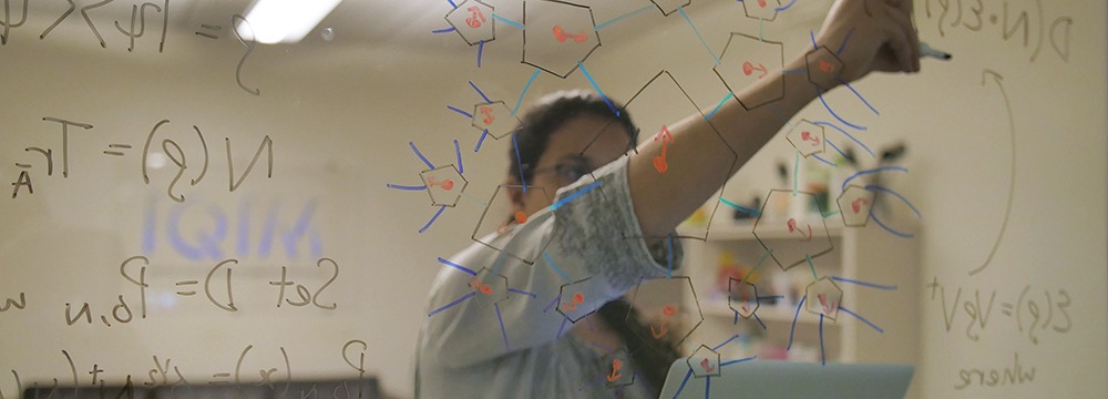
For AdS/CFT, suppose we are making a three-dimensional garment. The tailor of the universe never begins with three dimensions. Before him lies only the flat, two-dimensional fabric, with all its degrees of freedom spread upon the board.
It is then, in a less sartorial language, we might call the disentangling and entangling of degrees of freedom; the tailor coaxes a third dimension out of the flat cloth. This is the secret embroidery of the holographic idea: what appears to the wearer as a three-dimensional world is encoded in a fundamentally two-dimensional way.
Bob tries this newly fashioned quantum garment on before entering the black hole.
“Too tight,” he says. “See if there is more degree of freedom.”
The physicist frowns, takes up his chalk, and makes another small mark, with some disentangling and entangling here and there.
What could have been wrong? Well, perhaps the group theory has been chosen badly, the symmetry is broken, and a representation must be changed, a seam opened, a dimension added, or one cunningly concealed.
Alice watches him work, the almighty tailor of the universe, making change without a change.
“But how do you know when the suit is right?”
And with that, the physicist looks at her.
“What do you want? Do you want to put me out of work? Unknowing is the lack that drives us to make more suits. If we knew the suit was right, that would be the end of everything.”
 means “greater than”; and
  , “greater than or equal to.” Don’t translate
  and
and  .
. . Evolve it under
  …”).
…”). defines a regime, not a limit. The conditions
  and
and  define limits and are inequivalent to
  Then Y.”
 then Y.
 . Substituting into Eq. (1) yields [equation].
 ,
, 
 denote the measurement outcome.
 denote the Pauli-
 operator of qubit
 :
:
 , encoding directionality.
 -axis
-axis , which means
  to physicists. Use
  instead, unless you’re writing for engineers (who denote
  (\ell) instead.
 , –,
, –,  , or
, or  . Find the symbol immediately rightward of the initial = sign. Begin the new line directly below that symbol.
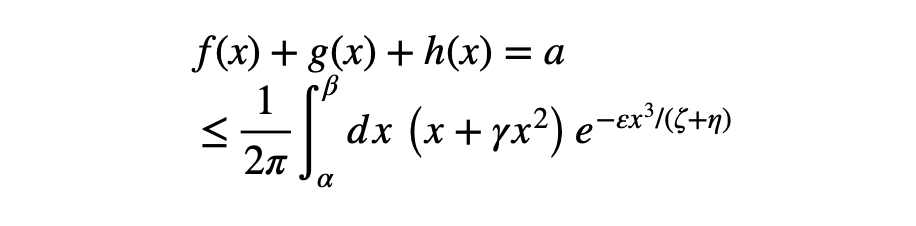
 in the example under (A). Put the corresponding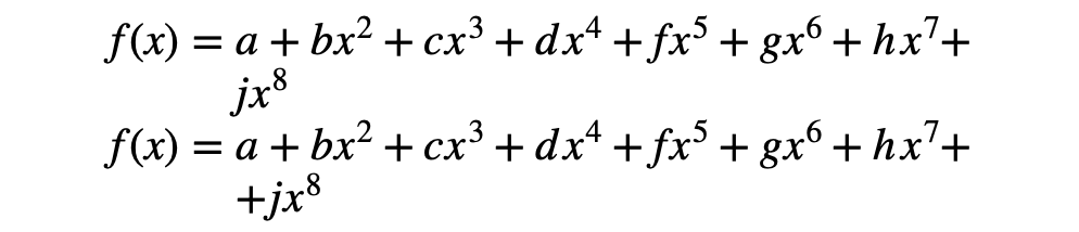
 means “approximately equals”; and ~, “scales as.” Approximations convey more information than scaling relations do.
 For example, if
  is odd, then
  and
and  fit the template.
 isn’t a matrix; a matrix represents an operator in terms of a particular basis. Therefore, no equals sign should interrelate an

 of real numbers
 and
and