
Justin Dressel’s office could understudy for the archetype of a physicist’s office. A long, rectangular table resembles a lab bench. Atop the table perches a tesla coil. A larger tesla coil perches on Justin’s desk. Rubik’s cubes and other puzzles surround a computer and papers. In front of the desk hangs a whiteboard.
A puzzle filled the whiteboard in August. Justin had written a model for a measurement of a quasiprobability. I introduced quasiprobabilities here last Halloween. Quasiprobabilities are to probabilities as ebooks are to books: Ebooks resemble books but can respond to touchscreen interactions through sounds and animation. Quasiprobabilities resemble probabilities but behave in ways that probabilities don’t.

A tesla coil of Justin Dressel’s
Let 

We can infer the tesla-coil probability by observing many physicists’ offices:

We could observe a quantum system weakly. We’d correlate our measurement device (the analogue of light) with the quantum state (the analogue of the tesla-coil number) unreliably. Imagining shining a dull light on an office for a brief duration. Shadows would obscure our photo. We’d have trouble inferring the number of tesla coils. But the dull, brief light burst would affect the office less than a strong, long burst would.
Justin explained how to infer a quasiprobability from weak measurements. He’d explained on account of an action that others might regard as weak: I’d asked for help.

Chaos had seized my attention a few weeks earlier. Chaos is a branch of math and physics that involves phenomena we can’t predict, like weather. I had forayed into quantum chaos for reasons I’ll explain in later posts. I was studying a function 
I’d derived a theorem about
“Is this amplitude physical?” John Preskill asked. “Can you measure it?”
“I don’t know,” I admitted. “I can tell a story about what it signifies.”
“If you could measure it,” he said, “I might be more excited.”
You needn’t study chaos to predict that private clouds drizzled on me that evening. I was grateful to receive feedback from thinkers I respected, to learn of a weakness in my argument. Still, scientific works are creative works. Creative works carry fragments of their creators. A weakness in my argument felt like a weakness in me. So I took the step that some might regard as weak—by seeking help.

Some problems, one should solve alone. If you wake me at 3 AM and demand that I solve the Schrödinger equation that governs a particle in a box, I should be able to comply (if you comply with my demand for justification for the need to solve the Schrödinger equation at 3 AM).4 One should struggle far into problems before seeking help.
Some scientists extend this principle into a ban on assistance. Some students avoid asking questions for fear of revealing that they don’t understand. Some boast about passing exams and finishing homework without the need to attend office hours. I call their attitude “scientific machismo.”
I’ve all but lived in office hours. I’ve interrupted lectures with questions every few minutes. I didn’t know if I could measure that probability amplitude. But I knew three people who might know. Twenty-five minutes after I emailed them, Justin replied: “The short answer is yes!”

I visited Justin the following week, at Chapman University’s Institute for Quantum Studies. I sat at his bench-like table, eyeing the nearest tesla coil, as he explained. Justin had recognized my probability amplitude from studies of the Kirkwood-Dirac quasiprobability. Experimentalists infer the Kirkwood-Dirac quasiprobability from weak measurements. We could borrow these experimentalists’ techniques, Justin showed, to measure my probability amplitude.
The borrowing grew into a measurement protocol. The theorem grew into a paper. I plunged into quasiprobabilities and weak measurements, following Justin’s advice. John grew more excited.
The meek might inherit the Earth. But the weak shall measure the quasiprobability.
With gratitude to Justin for sharing his expertise and time; and to Justin, Matt Leifer, and Chapman University’s Institute for Quantum Studies for their hospitality.
Chapman’s community was gracious enough to tolerate a seminar from me about thermal states of quantum systems. You can watch the seminar here.
1Tesla-coil collectors consists of atoms described by quantum theory. But we can describe tesla-coil collectors without quantum theory.
2Readers foreign to quantum theory can interpret “nonclassical” roughly as “quantum.”
3Debate has raged about whether quasiprobabilities govern classical phenomena.
4I should be able also to recite the solutions from memory.

In physics the probabilities that are represented by the wave function are generated by mechanisms (outside of the Hilbert space) that apply inhomogeneous spatial Poisson point processes. The characteristic function of the process equals the Fourier transform of the location density distribution that corresponds to the squared modulus of the wave function of the elementary particle that is served by the mechanism. The mechanism provides a Hilbert space operator with quaternionic eigenvalues. Therefore, after ordering of the real parts of the eigenvalues, the elementary particle appears to hop around in a stochastic hopping path ans after a while the hop landing locations have formed a location swarm that characterizes the particle and that conforms to the location density distribution. Since its Fourier transform exists the particle can show wave behavior and it owns a displacement generator. This means that at first approximation the swarm moves as one unit.
The hops initialize vibrations of the field that embeds the particle. These vibrations are sherical shape keeping fronts. After integration over a long enough period the result is the Green’s function of the field. When this is convoluted with the location density distribution then the deformation of the field due to the presence of the particle results.
TheHilbertBookTestModel by Hans van Leunen https://doc.co/WmxXCB
Pingback: It’s CHAOS! | Quantum Frontiers
Pingback: Local operations and Chinese communications | Quantum Frontiers
I’ve been thinking about this since I saw it a few days ago. In the notation in Justin’s 2015 PRA, he constructs the weak value as , which we can write using a projection operator
  as
as 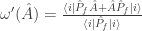 .
.  is a self-adjoint observable, so we can construct a protocol for measuring it. The trouble with this construction, for me, is that it is not a state over the algebra of observables, so that, in particular, what ought to be the variance of
  is not in general positive semi-definite. This is rather different than constructing a Wigner function for several non-commuting observables.
 followed by von Neumann measurement,
 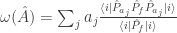 , which we can read as “the weak measurement result associated with
  , given the final von Neumann measurement $\latex f$”. Of course a weak von Neumann measurement is not no measurement at all, since it eliminates cross-terms (indeed I think of QM as not having an operation for “what the measurement result would have been if we could do the measurement without affecting the measured state at all”), but is there some other way of constructing a state, instead of a not-a-state, over the algebra of observables?
A more natural “weak” measurement, from a point of view that insists that we ought to construct a state over the algebra of observables, seems to be to use a weak von Neumann measurement, using the spectral decomposition of
Thanks again for your interest, Peter. For the rest of Quantum Frontiers’ readers: After Peter posted his comment, an email exchange took place amongst Peter, me, and Justin Dressel. I’m pasting the conversation here, with the writers’ permission, so that other QF readers can benefit.
– Nicole
—————————
Hi, Peter,
Thanks for your comment and email; I appreciate your taking the time to think about the matter. I’m copying Justin, with whom I’m finishing a follow-up to the paper mentioned in the post. At the moment, I’m buried in a late-stage proofread. I look forward to thinking about your message as soon as I reemerge into the real world!
Best wishes,
Nicole
———————
Hi Peter,
Glad to hear of your interest. If I understand your question correctly, you are wondering how to relate the formal weak value expression to a sensible state omega that properly averages the observable. Indeed, this has been the main source of contention about the weak value : It cannot correspond to a state in the usual sense. Nevertheless, it is a relevant value that consistently appears empirically as the limit point of a conditioned expectation value as the coupling strength tends to zero. This implies that it has robust structural significance, even though there is no obvious interpretation as a proper average of eigenvalues. This is where the quasiprobability perspective comes into play : There is a sense in which it is a conditioned average of eigenvalues, but only if you permit an extended notion of joint probability that allows negative or complex values. (The usual notion of state as a positive semidefinite probability functional over the observable algebra disallows this notion.)
Since you mentioned the Wigner distribution, I’ll point out that in the same 2015 paper I show how computing the conditioned average using the Wigner joint distribution yields the same quantity. So in some sense, it’s a stable quantity independent of the particular interpretation of the quasiprobabilities.
Personally, I find that it’s very easy to confuse these issues when just looking at how the formalism is written without empirical context. For example, you mentioned that the symmetric product of A with the postselection projector is an Hermitian observable that could be measured properly in its own right. That is formally true, but misses the main significance of the weak value as stably appearing during a straightforward estimation of A itself in the laboratory. That is, one constructs an unbiased estimation of A, which produces an ensemble of data that averages to its expectation value. Then one further tags that data with a second strong measurement after the first. Again, averaging everything still yields the total expectation value of A alone. However, using the additional tags of the second measurement, the ensemble of data can be partitioned into subensembles that can then be averaged separately. Remarkably, in the limit that the first measurement is weak, these subensemble averages always converge to weak values of A. This is true independent of measurement apparatus or any other specifics of the procedure, provided that the estimation procedure for A is unbiased (correctly yielding the expectation value when all data is averaged). It’s not obvious why there should be such a stable limit point for such conditioned averages, but the important thing is the simplicity of the empirical procedure : Measure A weakly and condition the ensemble in the usual way, and the weak value just appears in the data. In this sense it is not defined by its expression by the theorist a priori. Rather, the theorist must explain how to understand that expression given that it appears in the data unexpectedly.
Anyway, hope this helps clarify.
Cheers,
Justin
——————
Thanks, Justin,
A very interesting reply! I had been thinking that Wigner functions and this case are rather different, insofar as the marginal distributions for position and for momentum are, separately, perfectly reasonable probability distributions, whereas for this construction even the single-observable case does not generate a probability distribution, which is manifest in that even the “variance” might not be positive. I’ve now read Section IV B in your PRA 2015 carefully, and I see that the appearance of weak values in the Wigner function context appears not for marginals but, obviously, when conditioned for a given value of x or p. That now seems, indeed, so obvious! That leaves me with no worries, everything emerges naturally enough because there are non-commuting observables.
I find myself not too concerned about the theoretical construction. Given a Hilbert space of states, two privileged states |i〉 and |f〉, and an operator A, construct linear maps ω(A) into the complex numbers; there is only a limited range of such constructions. If ω(A*A)≥0 and ω(1)=1, we call ω(⋅) a state and we can talk about expectation values for An and the probability distribution associated with A, but in general not about joint probability distributions if we introduce a second operator B; if ω(⋅) is not a state, then we will not in general be able to talk about probability distributions.
I’m over-simplifying, a lot, insofar as you also introduce Hamiltonian interactions with measurement apparatuses, which introduces a much larger Hilbert space, but my head isn’t big enough to accommodate too much of that. Your last paragraph below is interesting in this respect, of course. I still find myself somewhat concerned that there is also available to us the somewhat natural weak measurement that I describe in the second paragraph of my comment on Nicole’s post, which seems a plausible alternative to your form of weak measurement. Your form of weak measurement seems not to modify the state as a QM measurement should, however I think I accept that your mathematics and your interpretation are both perfectly reasonable. Nonetheless, I suspect that you emerge with “such a stable limit point for such conditioned averages” because of the assumptions you make to construct them, which are apparently strong enough that you don’t ever emerge with “my” alternative.
I’ll take the liberty of commenting that Wigner functions do appear in classical signal analysis. Essentially, in signal analysis we use fourier analysis, so that Hilbert spaces are a natural mathematics, for which the fourier components of the signal and the position components of the signal are incompatible bases. For deterministic signal analysis, Leon Cohen, PROCEEDINGS OF THE IEEE, VOL. 77, NO. 7, JULY 1989, “Time-Frequency Distributions-A Review”, is a moderately effective review, although there is no mention of the Hilbert space perspective that I would prefer.
One can also go beyond the deterministic signal analysis case and make a connection between random fields and quantum fields, as I do in my “Equivalence of the Klein-Gordon random field and the complex Klein-Gordon quantum field”, EPL, 87 (2009) 31002 [the main reason not to like this paper, I suppose, is that it introduces positive and negative frequency components instead of the purely positive frequency components of quantum fields. A similar construction is possible for the EM field, but not for fermions, so that’s not so good either.]
All of which is to suggest that your last sentence in your Section IV B, “Such negativity, in turn, arises from intrinsic quantum interference that is not present in classical systems of particles,” may possibly be correct for particles, but for me is somewhat less correct for classical random fields.
In any case, I hope I notice the paper you’re writing with Nicole when it appears.
Best wishes,
Peter.
—————-
Hi Peter,
Yes, exactly! There is no reason we should be able to consider joint distributions for non-commuting observables, which is why joint quasi-probabilities appear as a (non-unique) compromise.
As far as your alternative definition using the spectral measure of A, that distribution will be physically correct for a sequence of strong measurements that are then conditioned (since the state collapses after the first measurement in that case). Aharonov, Bergmann, and Lebowitz wrote this down in 1964, though Watanabe was maybe first in 1955. The strange thing is that weakening the measurement continuously interpolates a conditioned average of data between that strong (classical) conditioned average and the weak value as extremal points of a deformation parameterized by the coupling strength. I show some examples of this interpolation in PRL 109, 230402 (2012) for several detector variations. It’s a curious situation.
And yes, I emphasize this point about classical wave-like fields in that same 2015 paper. It’s only weird if you detect discrete events! Waves have this structure already without issue. I pointed Nicole to the signal processing literature that indeed has developed all the quasiprobability distributions for joint time-frequency descriptions. Notably the Kirkwood-Dirac distribution was rediscovered there by Rihaczek and may be better known by that name.
It’s fun stuff!
———————
Dear Justin,
You have been so gentle with my naive comments! I apologize for them, but I’ve learned a lot in a very short time, so thanks again. I’ll reiterate that I found my restatement of as not-a-state, , helpful for me (because it’s more directly comparable with von Neumann and other measurements), at the same time as acknowledging your observation that this “is formally true, but misses the main significance of the weak value as stably appearing during a straightforward estimation of A itself in the laboratory”, but then also noting that an entirely counterfactual “straightforward estimation” might be best thought of as not-an-observable. Thanks also for the pointers to where my has, unsurprisingly, been thought of before.
It is fun stuff! I’m sadly more a “but” kind of person rather than an unalloyed “it’s fun stuff” sort of person, so I have to say (I don’t, but I do) that it feels like a sideshow to whatever the main event is. For me, the main event is for us to get a steadily better handle on quantum field theory, which over the last 5-10 years has come for me to be through a signal processing perspective on QFT. I’ve come to take the view that QFT is not badly understood as a linear and multilinear impulse-response formalism, with a crucial restriction to only the Lorentz-invariantly analytic-signal, positive-frequency component of the window or test function space. Recently, however, I have come to want to understand the relationship of such an abstract approach to actual measurement, for which Nicole’s pointer to your paper and your comments here have been very helpful.
I’m more than pleased that you have something of a sophisticated perspective of classical signal processing, since that’s something I’ve only rarely seen amongst people who have any focus on foundations. I’m very curious whether you have a go-to signal processing review, article, or book that you sent Nicole to? Good though I think it is, I’ve often wished for something a little different from the Leon Cohen review I linked to below.
It’s not a Tesla coil demo, but for my “outreach”, I present a very broad brush approach to quantum optics through a YouTube video that I posted as a result of a conversation with my daughter, 4’32” of “Quantum Mechanics: Event Thinking”, https://www.youtube.com/watch?v=frSL-BJTh90. For this there can be plenty of “but”, but six weeks after I made it I’m still kinda 70-30 in favor of its mostly empiricist slant and its characterization of lists of times of events as a lossy compression of electronic signals.
Best wishes,
Peter.
Thanks again for your interest in the OTOC quasiprobability, Peter. The paper that Justin, Brian Swingle, and I wrote about it has just appeared on the arXiv: https://arxiv.org/abs/1704.01971.
I saw, I have it downloaded, I shall read it.
Pingback: Glass beads and weak-measurement schemes | Quantum Frontiers
Pingback: Standing back at Stanford | Quantum Frontiers
Pingback: Paradise | Quantum Frontiers
Pingback: Gently yoking yin to yang | Quantum Frontiers
Pingback: Catching up with the quantum-thermo crowd | Quantum Frontiers
Pingback: I get knocked down… | Quantum Frontiers
Pingback: Doctrine of the (measurement) mean | Quantum Frontiers
Pingback: “A theorist I can actually talk with” | Quantum Frontiers
Pingback: Long live Yale’s cemetery | Quantum Frontiers
Pingback: Quantum conflict resolution | Quantum Frontiers
Pingback: Sense, sensibility, and superconductors | Quantum Frontiers
Pingback: If the (quantum-metrology) key fits… | Quantum Frontiers
Quasi probability seems like a phenomena appropriate for the quantum sociology questions of non causal interactions of the self and the non selves. It would be great to interact with the Chapmen University folks through a seminar or two.
Pingback: Life among the experimentalists | Quantum Frontiers
Pingback: Cutting the quantum mustard | Quantum Frontiers
Pingback: Eight highlights from publishing a science book for the general public | Quantum Frontiers