John Preskill, Richard P. Feynman Professor of Theoretical Physics at Caltech, has been named the 2024 John Stewart Bell Prize recipient. The prize honors John’s contributions in “the developments at the interface of efficient learning and processing of quantum information in quantum computation, and following upon long standing intellectual leadership in near-term quantum computing.” The committee cited John’s seminal work defining the concept of the NISQ (noisy intermediate-scale quantum) era, our joint work “Predicting Many Properties of a Quantum System from Very Few Measurements” proposing the classical shadow formalism, along with subsequent research that builds on classical shadows to develop new machine learning algorithms for processing information in the quantum world.
We are truly honored that our joint work on classical shadows played a role in John winning this prize. But as the citation implies, this is also a much-deserved “lifetime achievement” award. For the past two and a half decades, first at IQI and now at IQIM, John has cultivated a wonderful, world-class research environment at Caltech that celebrates intellectual freedom, while fostering collaborations between diverse groups of physicists, computer scientists, chemists, and mathematicians. John has said that his job is to shield young researchers from bureaucratic issues, teaching duties and the like, so that we can focus on what we love doing best. This extraordinary generosity of spirit has been responsible for seeding the world with some of the bests minds in the field of quantum information science and technology.
It is in this environment that the two of us (Robert and Richard) met and first developed the rudimentary form of classical shadows — inspired by Scott Aaronson’s idea of shadow tomography. While the initial form of classical shadows is mathematically appealing and was appreciated by the theorists (it was a short plenary talk at the premier quantum information theory conference), it was deemed too abstract to be of practical use. As a result, when we submitted the initial version of classical shadows for publication, the paper was rejected. John not only recognized the conceptual beauty of our initial idea, but also pointed us towards a direction that blossomed into the classical shadows we know today. Applications range from enabling scientists to more efficiently understand engineered quantum devices, speeding up various near-term quantum algorithms, to teaching machines to learn and predict the behavior of quantum systems.
Congratulations John! Thank you for bringing this community together to do extraordinarily fun research and for guiding us throughout the journey.
This past summer, our quantum thermodynamics research group had the wonderful opportunity to visit the Dibner Rare Book Library in D.C. Located in a small corner of the Smithsonian National Museum of American History, tucked away behind flashier exhibits, the Dibner is home to thousands of rare books and manuscripts, some dating back many centuries.
Our advisor, Nicole Yunger Halpern, has a special connection to the Dibner, having interned there as an undergrad. She’s remained in contact with the head librarian, Lilla Vekerdy. For our visit, the two of them curated a large spread of scientific work related to thermodynamics, physics, and mathematics. The tomes ranged from a 1500s print of Euclid’s Elements to originals of Einstein’s manuscripts with hand-written notes in the margin.
The print of Euclid’s Elements was one of the standout exhibits. It featured a number of foldout nets of 3D solids, which had been cut and glued into the book by hand. Several hundred copies of this print are believed to have been made, each of them containing painstakingly crafted paper models. At the time, this technique was an innovation, resulting from printers’ explorations of the then-young art of large-scale book publication.
Another interesting exhibit was rough notes on ideal gases written by Planck, one of the fathers of quantum mechanics. Ideal gases are the prototypical model in statistical mechanics, capturing to high accuracy the behaviour of real gases within certain temperatures and pressures. The notes contained comparisons between Boltzmann, Ehrenfest, and Planck’s own calculations for classical and quantum ideal gases. Though the prose was in German, some results were instantly recognizable, such as the plot of the specific heat of a classical ideal gas, showing the stepwise jump as degrees of freedom freeze out.
Looking through these great physicists’ rough notes, scratched-out ideas, and personal correspondences was a unique experience, helping humanize them and place their work in historical context. Understanding the history of science doesn’t just need to be for historians, it can be useful for scientists themselves! Seeing how scientists persevered through unknowns, grappling with doubts and incomplete knowledge to generate new ideas, is inspiring. But when one only reads the final, polished result in a modern textbook, it can be difficult to appreciate this process of discovery. Another reason to study the historical development of scientific results is that core concepts have a way of arising time and again across science. Recognizing how these ideas have arisen in the past is insightful. Examining the creative processes of great scientists before us helps develop our own intuition and skillset.
Thanks to our advisor for this field trip – and make sure to check out the Dibner next time you’re in DC!
This is the first part in a four part series covering the recent Perspectives article on noncommuting charges. I’ll be posting one part every ~6 weeks leading up to my PhD thesis defence.
Thermodynamics problems have surprisingly many similarities with fairy tales. For example, most of them begin with a familiar opening. In thermodynamics, the phrase “Consider an isolated box of particles” serves a similar purpose to “Once upon a time” in fairy tales—both serve as a gateway to their respective worlds. Additionally, both have been around for a long time. Thermodynamics emerged in the Victorian era to help us understand steam engines, while Beauty and the Beast and Rumpelstiltskin, for example, originated about 4000 years ago. Moreover, each conclude with important lessons. In thermodynamics, we learn hard truths such as the futility of defying the second law, while fairy tales often impart morals like the risks of accepting apples from strangers. The parallels go on; both feature archetypal characters—such as wise old men and fairy godmothers versus ideal gases and perfect insulators—and simplified models of complex ideas, like portraying clear moral dichotomies in narratives versus assuming non-interacting particles in scientific models.1
Of all the ways thermodynamic problems are like fairytale, one is most relevant to me: both have experienced modern reimagining. Sometimes, all you need is a little twist to liven things up. In thermodynamics, noncommuting conserved quantities, or charges, have added a twist.
Unfortunately, my favourite fairy tale, ‘The Hunchback of Notre-Dame,’ does not start with the classic opening line ‘Once upon a time.’ For a story that begins with this traditional phrase, ‘Cinderella’ is a great choice.
First, let me recap some of my favourite thermodynamic stories before I highlight the role that the noncommuting-charge twist plays. The first is the inevitability of the thermal state. For example, this means that, at most times, the state of most sufficiently small subsystem within the box will be close to a specific form (the thermal state).
The second is an apparent paradox that arises in quantum thermodynamics: How do the reversible processes inherent in quantum dynamics lead to irreversible phenomena such as thermalization? If you’ve been keeping up with Nicole Yunger Halpern‘s (my PhD co-advisor and fellow fan of fairytale) recent posts on the eigenstate thermalization hypothesis (ETH) (part 1 and part 2) you already know the answer. The expectation value of a quantum observable is often comprised of a sum of basis states with various phases. As time passes, these phases tend to experience destructive interference, leading to a stable expectation value over a longer period. This stable value tends to align with that of a thermal state’s. Thus, despite the apparent paradox, stationary dynamics in quantum systems are commonplace.
The third story is about how concentrations of one quantity can cause flows in another. Imagine a box of charged particles that’s initially outside of equilibrium such that there exists gradients in particle concentration and temperature across the box. The temperature gradient will cause a flow of heat (Fourier’s law) and charged particles (Seebeck effect) and the particle-concentration gradient will cause the same—a flow of particles (Fick’s law) and heat (Peltier effect). These movements are encompassed within Onsager’s theory of transport dynamics…if the gradients are very small. If you’re reading this post on your computer, the Peltier effect is likely at work for you right now by cooling your computer.
What do various derivations of the thermal state’s forms, the eigenstate thermalization hypothesis (ETH), and the Onsager coefficients have in common? Each concept is founded on the assumption that the system we’re studying contains charges that commute with each other (e.g. particle number, energy, and electric charge). It’s only recently that physicists have acknowledged that this assumption was even present.
This is important to note because not all charges commute. In fact, the noncommutation of charges leads to fundamental quantum phenomena, such as the Einstein–Podolsky–Rosen (EPR) paradox, uncertainty relations, and disturbances during measurement. This raises an intriguing question. How would the above mentioned stories change if we introduce the following twist?
“Consider an isolated box with charges that do not commute with one another.”
This question is at the core of a burgeoning subfield that intersects quantum information, thermodynamics, and many-body physics. I had the pleasure of co-authoring a recent perspective article in Nature Reviews Physics that centres on this topic. Collaborating with me in this endeavour were three members of Nicole’s group: the avid mountain climber, Billy Braasch; the powerlifter, Aleksander Lasek; and Twesh Upadhyaya, known for his prowess in street basketball. Completing our authorship team were Nicole herself and Amir Kalev.
To give you a touchstone, let me present a simple example of a system with noncommuting charges. Imagine a chain of qubits, where each qubit interacts with its nearest and next-nearest neighbours, such as in the image below.
The figure is courtesy of the talented team at Nature. Two qubits form the system S of interest, and the rest form the environment E. A qubit’s three spin components, σa=x,y,z, form the local noncommuting charges. The dynamics locally transport and globally conserve the charges.
In this interaction, the qubits exchange quanta of spin angular momentum, forming what is known as a Heisenberg spin chain. This chain is characterized by three charges which are the total spin components in the x, y, and z directions, which I’ll refer to as Qx, Qy, and Qz, respectively. The Hamiltonian H conserves these charges, satisfying [H, Qa] = 0 for each a, and these three charges are non-commuting, [Qa, Qb] ≠ 0, for any pair a, b ∈ {x,y,z} where a≠b. It’s noteworthy that Hamiltonians can be constructed to transport various other kinds of noncommuting charges. I have discussed the procedure to do so in more detail here (to summarize that post: it essentially involves constructing a Koi pond).
This is the first in a series of blog posts where I will highlight key elements discussed in the perspective article. Motivated by requests from peers for a streamlined introduction to the subject, I’ve designed this series specifically for a target audience: graduate students in physics. Additionally, I’m gearing up to defending my PhD thesis on noncommuting-charge physics next semester and these blog posts will double as a fun way to prepare for that.
This opening text was taken from the draft of my thesis. ↩︎
Terry Rudolph, PsiQuantum & Imperial College London
During a recent visit to the wild western town of Pasadena I got into a shootout at high-noon trying to explain the nuances of this question to a colleague. Here is a more thorough (and less risky) attempt to recover!
tl;dr Photonic quantum computers can perform a useful computation orders of magnitude faster than a superconducting qubit machine. Surprisingly, this would still be true even if every physical timescale of the photonic machine was an order of magnitude longer (i.e. slower) than those of the superconducting one. But they won’t be.
SUMMARY
There is a misconception that the slow rate of entangled photon production from many current (“postselected”) experiments is somehow relevant to the logical speed of a photonic quantum computer. It isn’t, because those experiments don’t use an optical switch.
If we care about how fast we can solve useful problems then photonic quantum computers will eventually win that race. Not only because in principle their components can run faster, but because of fundamental architectural flexibilities which mean they need to do fewer things.
Unlike most quantum systems for which relevant physical timescales are determined by “constants of nature” like interaction strengths, the relevant photonic timescales are determined by “classical speeds” (optical switch speeds, electronic signal latencies etc). Surprisingly, even if these were slower – which there is no reason for them to be – the photonic machine can still compute faster.
In a simple world the speed of a photonic quantum computer would just be the speed at which it’s possible to make small (fixed sized) entangled states. GHz rates for such are plausible and correspond to the much slower MHz code-cycle rates of a superconducting machine. But we want to leverage two unique photonic features: Availability of long delays (e.g. optical fiber) and ease of nonlocal operations, and as such the overall story is much less simple.
If what floats your boat are really slow things, like cold atoms, ions etc., then the hybrid photonic/matter architecture outlined here is the way you can build a quantum computer with a faster logical gate speed than (say) a superconducting qubit machine. You should be all over it.
Magnifying the number of logical qubits in a photonic quantum computer by 100 could be done simply by making optical fiber 100 times less lossy. There are reasons to believe that such fiber is possible (though not easy!). This is just one example of the “photonics is different, photonics is different, ” mantra we should all chant every morning as we stagger out of bed.
The flexibility of photonic architectures means there is much more unexplored territory in quantum algorithms, compiling, error correction/fault tolerance, system architectural design and much more. If you’re a student you’d be mad to work on anything else!
Sorry, I realize that’s kind of an in-your-face list, some of which is obviously just my opinion! Lets see if I can make it yours too 🙂
I am not going to reiterate all the standard stuff about how photonics is great because of how manufacturable it is, its high temperature operation, easy networking modularity blah blah blah. That story has been told many times elsewhere. But there are subtleties to understanding the eventual computational speed of a photonic quantum computer which have not been explained carefully before. This post is going to slowly lead you through them.
I will only be talking about useful, large-scale quantum computing – by which I mean machines capable of, at a minimum, implementing billions of logical quantum gates on hundreds of logical qubits.
PHYSICAL TIMESCALES
In a quantum computer built from matter – say superconducting qubits, ions, cold atoms, nuclear/electronic spins and so on, there is always at least one natural and inescapable timescale to point to. This typically manifests as some discrete energy levels in the system, the levels that make the two states of the qubit. Related timescales are determined by the interaction strengths of a qubit with its neighbors, or with external fields used to control it. One of the most important timescales is that of measurement – how fast can we determine the state of the qubit? This generally means interacting with the qubit via a sequence of electromagnetic fields and electronic amplification methods to turn quantum information classical. Of course, measurements in quantum theory are a pernicious philosophical pit – some people claim they are instantaneous, others that they don’t even happen! Whatever. What we care about is: How long does it take for a readout signal to get to a computer that records the measurement outcome as classical bits, processes them, and potentially changes some future action (control field) interacting with the computer?
For building a quantum computer from optical frequency photons there are no energy levels to point to. The fundamental qubit states correspond to a single photon being either “here” or “there”, but we cannot trap and hold them at fixed locations, so unlike, say, trapped atoms these aren’t discrete energy eigenstates. The frequency of the photons does, in principle, set some kind of timescale (by energy-time uncertainty), but it is far too small to be constraining. The most basic relevant timescales are set by how fast we can produce, control (switch) or detect the photons. While these depend on the bandwidth of the photons used – itself a very flexible design choice – typical components operate in GHz regimes. Another relevant timescale is that we can store photons in a standard optical fiber for tens of microseconds before its probability of getting lost exceeds (say) 10%.
There is a long chain of things that need to be strung together to get from component-level physical timescales to the computational speed of a quantum computer built from them. The first step on the journey is to delve a little more into the world of fault tolerance.
TIMESCALES RELEVANT FOR FAULT TOLERANCE
The timescales of measurement are important because they determine the rate at which entropy can be removed from the system. All practical schemes for fault tolerance rely on performing repeated measurements during the computation to combat noise and imperfection. (Here I will only discuss surface-code fault tolerance, much of what I say though remains true more generally.) In fact, although at a high level one might think a quantum computer is doing some nice unitary logic gates, microscopically the machine is overwhelmingly just a device for performing repeated measurements on small subsets of qubits.
In matter-based quantum computers the overall story is relatively simple. There is a parameter , the “code distance”, dependent primarily on the quality of your hardware, which is somewhere in the range of 20-40. It takes qubits to make up a logical qubit, so let’s say 1000 of them per logical qubit. (We need to make use of an equivalent number of ancillary qubits as well). Very roughly speaking, we repeat twice the following: each physical qubit gets involved in a small number (say 4-8) of two-qubit gates with neighboring qubits, and then some subset of qubits undergo a single-qubit measurement. Most of these gates can happen simultaneously, so (again, roughly!) the time for this whole process is the time for a handful of two-qubit gates plus a measurement. It is known as a code cycle and the time it takes we denote . For example, in superconducting qubits this timescale is expected to be about 1 microsecond, for ion-trap qubits about 1 millisecond. Although variations exist, lets stick to considering a basic architecture which requires repeating this whole process on the order of times in order to complete one logical operation (i.e., a logical gate). So, the time for a logical gate would be , this sets the effective logical gate speed.
If you zoom out, each code cycle for a single logical qubit is therefore built up in a modular fashion from copies of the same simple quantum process – a process that involves a handful of physical qubits and gates over a handful of time steps, and which outputs a classical bit of information – a measurement outcome. I have ignored the issue of what happens to those measurement outcomes. Some of them will be sent to a classical computer and processed (decoded) then fed back to control systems and so on. That sets another relevant timescale (the reaction time) which can be of concern in some approaches, but early generations of photonic machines – for reasons outlined later – will use long delay lines, and it is not going to be constraining.
In a photonic quantum computer we also build up a single logical qubit code cycle from copies of some quantum stuff. In this case it is from copies of an entangled state of photons that we call a resource state. The number of entangled photons comprising one resource state depends a lot on how nice and clean they are, lets fix it and say we need a 20-photon entangled state. (The noisier the method for preparing resource states the larger they will need to be). No sequence of gates is performed on these photons. Rather, photons from adjacent resource states get interfered at a beamsplitter and immediately detected – a process we call fusion. You can see a toy version in this animation:
Highly schematic depiction of photonic fusion based quantum computing. An array of 25 resource state generators each repeatedly create resource states of 6 entangled photons, depicted as a hexagonal ring. Some of the photons in each ring are immediately fused (the yellow flashes) with photons from adjacent resource states, the fusion measurement outputs classical bits of information. One photon from each ring gets delayed for one clock cycle and fused with a photon from the next clock cycle.
Measurements destroy photons, so to ensure continuity from one time step to the next some photons in a resource state get delayed by one time step to fuse with a photon from the subsequent resource state – you can see the delayed photons depicted as lit up single blobs if you look carefully in the animation.
The upshot is that the zoomed out view of the photonic quantum computer is very similar to that of the matter-based one, we have just replaced the handful of physical qubits/gates of the latter with a 20-photon entangled state. (And in case it wasn’t obvious – building a bigger computer to do a larger computation means generating more of the resource states, it doesn’t mean using larger and larger resource states.)
If that was the end of the story it would be easy to compare the logical gate speeds for matter-based and photonic approaches. We would only need to answer the question “how fast can you spit out and measure resource states?”. Whatever the time for resource state generation, , the time for a logical gate would be and the photonic equivalent of would simply be . (Measurements on photons are fast and so the fusion time becomes effectively negligible compared to .) An easy argument could then be made that resource state generation at GHz rates is possible, therefore photonic machines are going to be orders of magnitude faster, and this article would be done! And while I personally do think its obvious that one day this is where the story will end, in the present day and age….
… there are two distinct ways in which this picture is far too simple.
FUNKY FEATURES OF PHOTONICS, PART I
The first over-simplification is based on facing up to the fact that building the hardware to generate a photonic resource state is difficult and expensive. We cannot afford to construct one resource state generator per resource state required at each time step. However, in photonics we are very fortunate that it is possible to store/delay photons in long lengths of optical fiber with very low error rates. This lets us use many resource states all produced by a single resource state generator in such a way that they can all be involved in the same code-cycle. So, for example, all resource states required for a single code cycle may come from a single resource state generator:
Here the 25 resource state generators of the previous figure are replaced by a single generator that “plays fusion games with itself” by sending some of its output photons into either a delay of length 5 or one of length 25 times the basic clock cycle. We achieve a massive amplification of photonic entanglement simply by increasing the length of optical fiber used. By mildly increasing the complexity of the switching network a photon goes through when it exits the delay, we can also utilize small amounts of (logarithmic) nonlocal connectivity in the network of fusions performed (not depicted), which is critical to doing active volume compiling (discussed later).
You can see an animation of how this works in the figure – a single resource state generator spits out resource states (depicted again as a 6-qubit hexagonal ring), and you can see a kind of spacetime 3d-printing of entanglement being performed. We call this game interleaving. In the toy example of the figure we see some of the qubits get measured (fused) immediately, some go into a delay of length and some go into a delay of length .
So now we have brought another timescale into the photonics picture, the length of time that some photons spend in the longest interleaving delay line. We would like to make this as long as possible, but the maximum time is limited by the loss in the delay (typically optical fiber) and the maximum loss our error correcting code can tolerate. A number to have in mind for this (in early machines) is a handful of microseconds – corresponding to a few Km of fiber.
The upshot is that ultimately the temporal quantity that matters most to us in photonic quantum computing is:
What is the total number of resource states produced per second?
It’s important to appreciate we care only about the total rate of resource state production across the whole machine – so, if we take the total number of resource state generators we have built, and divide by , we get this total rate of resource state generation that we denote . Note that this rate is distinct from any physical clock rate, as, e.g., 100 resource state generators running at 100MHz, or 10 resource state generators running at 1GHz, or 1 resource state generator running at 10GHz all yield the same total rate of resource state production
The second most important temporal quantity is , the time of the longest low-loss delay we can use.
We then have that the total number of logical qubits in the machine is:
You can see this is proportional to which is effectively the total number of resource states “alive” in the machine at any given instant of time, including all the ones stacked up in long delay lines. This is how we leverage optical fiber delays for a massive amplification of the entanglement our hardware has available to compute with.
The time it takes to perform a logical gate is determined both by and by the total number of resource states that we need to consume for every logical qubit to undergo a gate. Even logical qubits that appear to not be part of a gate in that time step do, in fact, undergo a gate – the identity gate – because they need to be kept error free while they “idle”. As such the total number of resource states consumed in a logical time step is just and the logical gate time of the machine is
.
Because is expected to be about the same as for superconducting qubits (microseconds), the logical gate speeds are comparable.
At least they are, until…………
FUNKY FEATURES OF PHOTONICS, PART II
But wait! There’s more.
The second way in which unique features of photonics play havoc with the simple comparison to matter-based systems is in the exciting possibility of what we call an active-volume architecture.
A few moments ago I said:
Even logical qubits that seem to not be part of a gate in that time step undergo a gate – the identity gate – because they need to be kept error free while they “idle”. As such the total number of resource states consumed is just
and that was true. Until recently.
It turns out that there is a way of eliminating the majority of consumption of resources expended on idling qubits! This is done by some clever tricks that make use of the possibility of performing a limited number of non-nearest neighbor fusions between photons. It’s possible because photons are not anyway stuck in one place, and they can be passed around readily without interacting with other photons. (Their quantum crosstalk is exactly zero, they do really seem to despise each other.)
What previously was a large volume of resource states being consumed for “thumb-twiddling”, can instead all be put to good use doing non-trivial computational gates. Here is a simple quantum circuit with what we mean by the active volume highlighted:
Now, for any given computation the amount of active volume will depend very much on what you are computing. There are always many different circuits decomposing a given computation, some will use more active volume than others. This makes it impossible to talk about “what is the logical gate speed” completely independent of considerations about the computation actually being performed.
In this recent paper https://arxiv.org/abs/2306.08585 Daniel Litinski considers breaking elliptic curve cryptosystems on a quantum computer. In particular, he considers what it would take to run the relevant version of Shor’s algorithm on a superconducting qubit architecture with a microsecond code cycle – the answer is roughly that with 10 million physical superconducting qubits it would take about 4 hours (with an equivalent ion trap computer the time balloons to more than 5 months).
He then compares solving the same problem on a machine with an active volume architecture. Here is a subset of his results:
Recall that is the photonics parameter which is roughly equivalent to the code cycle time. Thus taking 1 microsecond compares to the expected for superconducting qubits. Imagine we can produce resource states at . This could be 6000 resource state generators each producing resource states at or 3500 generators producing them at 1GHz for example. Then the same computation would take 58 seconds, instead of four hours, a speedup by a factor of more than 200!
Now, this whole blog post is basically about addressing confusions out there regarding physical versus computational timescales. So, for the sake of illustration, let me push a purely theoretical envelope: What if we can’t do everything as fast as in the example just stated? What if our rate of total resource state generation was 10 times slower, i.e. ? And what if our longest delay is ten times longer, i.e. microseconds (so as to be much slower than )? Furthermore, for the sake of illustration, lets consider a ridiculously slow machine that achieves by building 350 billion resource state generators that can each produce resource states at only 1Hz. Yes, you read that right.
The fastest device in this ridiculous machine would only need to be a (very large!) slow optical switch operating at 100KHz (due to the chosen ). And yet this ridiculous machine could still solve the problem that takes a superconducting qubit machine four hours, in less than 10 minutes.
To reiterate:
Despite all the “physical stuff going on” in this (hypothetical, active-volume) photonic machine running much slower than all the “physical stuff going on” in the (hypothetical, non-active-volume) superconducting qubit machine, we see the photonic machine can still do the desired computation 25 times faster!
Hopefully the fundamental murkiness of the titular question “what is the logical gate speed of a photonic quantum computer” is now clear! Put simply: Even if it did “fundamentally run slower” (it won’t), it would still be faster. Because it has less stuff to do. It’s worth noting that the 25x increase in speed is clearly not based on physical timescales, but rather on the efficient parallelization achieved through long-range connections in the photonic active-volume device. If we were to scale up the hypothetical 10-million-superconducting-qubit device by a factor of 25, it could potentially also complete computations 25 times faster. However, this would require a staggering 250 million physical qubits or more. Ultimately, the absolute speed limit of quantum computations is set by the reaction time, which refers to the time it takes to perform a layer of single-qubit measurements and some classical processing. Early-generation machines will not be limited by this reaction time, although eventually it will dictate the maximum speed of a quantum computation. But even in this distant-future scenario, the photonic approach remains advantageous. As classical computation and communication speed up beyond the microsecond range, slower physical measurements of matter-based qubits will hinder the reaction time, while fast single-photon detectors won’t face the same bottleneck.
In the standard photonic architecture we saw that would scale proportionally with – that is, adding long delays would slow the logical gate speed (while giving us more logical qubits). But remarkably the active-volume architecture allows us to exploit the extra logical qubits without incurring a big negative tradeoff. I still find this unintuitive and miraculous, it just seems to so massively violate Conservation of Trouble.
With all this in mind it is also worth noting as an aside that optical fibers made from (expensive!) exotic glasses or with funky core structures are theoretically calculated to be possible with up to 100 times less loss than conventional fiber – therefore allowing for an equivalent scaling of . How many approaches to quantum computing can claim that perhaps one day, by simply swapping out some strands of glass, they could instantaneously multiply the number of logical qubits in the machine from (say) 100 to 10000? Even a (more realistic) factor of 10 would be incredible.
Obviously for pedagogical reasons the above discussion is based around the simplest approaches to logic in both standard and active-volume architectures, but more detailed analysis shows that conclusions regarding total computational time speedup persist even after known optimizations for both approaches.
Now the reason I called the example above a “ridiculous machine” is that even I am not cruel enough to ask our engineers to assemble 350 billion resource state generators. Fewer resource state generators running faster is desirable from the perspective of both sweat and dollars.
We have arrived then at a simple conclusion: what we really need to know is “how fast and at what scale can we generate resource states, with as large a machine as we can afford to build”.
HOW FAST COULD/SHOULD WE AIM TO DO RESOURCE STATE GENERATION?
In the world of classical photonics – such as that used for telecoms, LIDAR and so on – very high speeds are often thrown around: pulsed lasers and optical switches readily run at 100’s of GHz for example. On the quantum side, if we produce single photons via a probabilistic parametric process then similarly high repetition rates have been achieved. (This is because in such a process there are no timescale constraints set by atomic energy levels etc.) Off-the-shelf single photon avalanche photodiode detectors can count photons at multiple GHz.
Seems like we should be aiming to generate resource states at 10’s of GHz right?
Well, yes, one day – one of the main reasons I believe the long-term future of quantum computing is ultimately photonic is because of the obvious attainability of such timescales. [Two others: it’s the only sensible route to a large-scale room temperature machine; eventually there is only so much you can fit in a single cryostat, so ultimately any approach will converge to being a network of photonically linked machines].
In the real world of quantum engineering there are a couple of reasons to slow things down: (i) It relaxes hardware tolerances, since it makes it easier to get things like path lengths aligned, synchronization working, electronics operating in easy regimes etc (ii) in a similar way to how we use interleaving during a computation to drastically reduce the number of resource state generators we need to build, we can also use (shorter than length) delays to reduce the amount of hardware required to assemble the resource states in the first place and (iii) We want to use multiplexing.
Multiplexing is often misunderstood. The way we produce the requisite photonic entanglement is probabilistic. Producing the whole 20-photon resource state in a single step, while possible, would have very low probability. The way to obviate this is to cascade a couple of higher probability, intermediate, steps – selecting out successes (more on this in the appendix). While it has been known since the seminal work of Knill, Laflamme and Milburn two decades ago that this is a sensible thing to do, the obstacle has always been the need for a high performance (fast, low loss) optical switch. Multiplexing introduces a new physical “timescale of convenience” – basically dictated by latencies of electronic processing and signal transmission.
The brief summary therefore is: Yeah, everything internal to making resource states can be done at GHz rates, but multiple design flexibilities mean the rate of resource state generation is itself a parameter that should be tuned/optimized in the context of the whole machine, it is not constrained by fundamental quantum things like interaction energies, rather it is constrained by the speeds of a bunch of purely classical stuff.
I do not want to leave the impression that generation of entangled photons can only be done via the multistage probabilistic method just outlined. Using quantum dots, for example, people can already demonstrate generation of small photonic entangled states at GHz rates (see e.g. https://www.nature.com/articles/s41566-022-01152-2). Eventually, direct generation of photonic entanglement from matter-based systems will be how photonic quantum computers are built, and I should emphasize that its perfectly possible to use small resource states (say, 4 entangled photons) instead of the 20 proposed above, as long as they are extremely clean and pure. In fact, as the discussion above has hopefully made clear: for quantum computing approaches based on fundamentally slow things like atoms and ions, transduction of matter-based entanglement into photonic entanglement allows – by simply scaling to more systems – evasion of the extremely slow logical gate speeds they will face if they do not do so.
Right now, however, approaches based on converting the entanglement of matter qubits into photonic entanglement are not nearly clean enough, nor manufacturable at large enough scales, to be compatible with utility-scale quantum computing. And our present method of state generation by multiplexing has the added benefit of decorrelating many error mechanisms that might otherwise be correlated if many photons originate from the same device.
So where does all this leave us?
I want to build a useful machine. Lets back-of-the-envelope what that means photonically. Consider we target a machine comprising (say) at least 100 logical qubits capable of billions of logical gates. (From thinking about active volume architectures I learn that what I really want is to produce as many “logical blocks” as possible, which can then be divvied up into computational/memory/processing units in funky ways, so here I’m really just spitballing an estimate to give you an idea).
Staring at
and presuming and is going to be about 10 microseconds, we need to be producing resource states at a total rate of at least . As I hope is clear by now, as a pure theoretician, I don’t give a damn if that means 10000 resource state generators running at 1MHz, 100 resource state generators running at 100MHz, or 10 resource state generators running at 1GHz. However, the fact this flexibility exists is very useful to my engineering colleagues – who, of course, aim to build the smallest and fastest possible machine they can, thereby shortening the time until we let them head off for a nice long vacation sipping mezcal margaritas on a warm tropical beach.
None of these numbers should seem fundamentally indigestible, though I do not want to understate the challenge: all never-before-done large-scale engineering is extremely hard.
But regardless of the regime we operate in, logical gate speeds are not going to be the issue upon which photonics will be found wanting.
REAL-WORLD QUANTUM COMPUTING DESIGN
Now, I know this blog is read by lots of quantum physics students. If you want to impact the world, working in quantum computing really is a great way to do it. The foundation of everything round you in the modern world was laid in the 40’s and 50’s when early mathematicians, computer scientists, physicists and engineers figured out how we can compute classically. Today you have a unique opportunity to be part of laying the foundation of humanity’s quantum computing future. Of course, I want the best of you to work on a photonic approach specifically (I’m also very happy to suggest places for the worst of you to go work). Please appreciate, therefore, that these final few paragraphs are my very biased – though fortunately totally correct – personal perspective!
The broad features of the photonic machine described above – it’s a network of stuff to make resource states, stuff to fuse them, and some interleaving modules, has been fixed now for several years (see the references).
Once we go down even just one level of detail, a myriad of very-much-not-independent questions arise: What is the best resource state? What series of procedures is optimal for creating that state? What is the best underlying topological code to target? What fusion network can build that code? What other things (like active volume) can exploit the ability for photons to be easily nonlocally connected? What types of encoding of quantum information into photonic states is best? What interferometers generate the most robust small entangled states? What procedures for systematically growing resource states from smaller entangled states are most robust or use the least amount of hardware? How can we best use measurements and classical feedforward/control to mitigate error accumulation?
Those sorts of questions cannot be meaningfully addressed without going down to another level of detail, one in which we do considerable modelling of the imperfect devices from which everything will be built – modelling that starts by detailed parameterization of about 40 component specifications (ranging over things like roughness of silicon photonic waveguide walls, stability of integrated voltage drivers, precision of optical fiber cutting robots,….. Well, the list goes on and on). We then model errors of subsystems built from those components, verify against data, and proceed.
The upshot is none of these questions have unique answers! There just isn’t “one obviously best code” etc. In fact the answers can change significantly with even small variations in performance of the hardware. This opens a very rich design space, where we can establish tradeoffs and choose solutions that optimize a wide variety of practical hardware metrics.
In photonics there is also considerably more flexibility and opportunity than with most approaches on the “quantum side” of things. That is, the quantum aspects of the sources, the quantum states we use for encoding even single qubits, the quantum states we should target for the most robust entanglement, the topological quantum logical states we target and so on, are all “on the table” so to speak.
Exploring the parameter space of possible machines to assemble, while staying fully connected to component level hardware performance, involves both having a very detailed simulation stack, and having smart people to help find new and better schemes to test in the simulations. It seems to me there are far more interesting avenues for impactful research than more established approaches can claim. Right now, on this planet, there are only around 30 people engaged seriously in that enterprise. It’s fun. Perhaps you should join in?
REFERENCES
A surface code quantum computer in siliconhttps://www.science.org/doi/10.1126/sciadv.1500707. Figure 4 is a clear depiction of the circuits for performing a code cycle appropriate to a generic 2d matter-based architecture.
Here is a common misconception: Current methods of producing ~20 photon entangled states succeed only a few times per second, so generating resource states for fusion-based quantum computing is many orders of magnitude away from where it needs to be.
This misconception arises from considering experiments which produce photonic entangled states via single-shot spontaneous processes and extrapolating them incorrectly as having relevance to how resource states for photonic quantum computing are assembled.
Such single-shot experiments are hit by a “double whammy”. The first whammy is that the experiments produce some very large and messy state that only has a tiny amplitude in the component of the desired entangled state. Thus, on each shot, even in ideal circumstances, the probability of getting the desired state is very, very small. Because billions of attempts can be made each second (as mentioned, running these devices at GHz speeds is easy) it does occasionally occur. But only a small number of times per second.
The second whammy is that if you are trying to produce a 20-photon state, but each photon gets lost with probability 20%, then the probability of you detecting all the photons – even if you live in a branch of the multiverse where they have been produced – is reduced by a factor of . Loss reduces the rate of production considerably.
Now, photonic fusion-based quantum computing could not be based on this type of entangled photon generation anyway, because the production of the resource states needs to be heralded, while these experiments only postselect onto the very tiny part of the total wavefunction with the desired entanglement. But let us put that aside, because the two whammy’s could, in principle, be showstoppers for production of heralded resource states, and it is useful to understand why they are not.
Imagine you can toss coins, and you need to generate 20 coins showing Heads. If you repeatedly toss all 20 coins simultaneously until they all come up heads you’d typically have to do so millions of times before you succeed. This is even more true if each coin also has a 20% chance of rolling off the table (akin to photon loss). But if you can toss 20 coins, set aside (switch out!) the ones that came up heads and re-toss the others, then after only a small number of steps you will have 20 coins all showing heads. This large gap is fundamentally why the first whammy is not relevant: To generate a large photonic entangled state we begin by probabilistically attempting to generate a bunch of small ones. We then select out the success (multiplexing) and combine successes to (again, probabilistically) generate a slightly larger entangled state. We repeat a few steps of this. This possibility has been appreciated for more than twenty years, but hasn’t been done at scale yet because nobody has had a good enough optical switch until now.
The second whammy is taken care of the fact that for fault tolerant photonic fusion-based quantum computing there never is any need to make the resource state such that all photons are guaranteed to be there! The per-photon loss rate can be high (in principle 10’s of percent) – in fact the larger the resource state being built the higher it is allowed to be.
The upshot is that comparing this method of entangled photon generation with the methods which are actually employed is somewhat like a creation scientist claiming monkeys cannot have evolved from bacteria, because it is all so unlikely for suitable mutations to have happened simultaneously!
Acknowledgements
Very grateful to Mercedes Gimeno-Segovia, Daniel Litinski, Naomi Nickerson, Mike Nielsen and Pete Shadbolt for help and feedback.
By guest blogger Clarice D. Aiello, faculty at UCLA
Imagine using your cellphone to control the activity of your own cells to treat injuries and disease. It sounds like something from the imagination of an overly optimistic science fiction writer. But this may one day be a possibility through the emerging field of quantum biology.
Over the past few decades, scientists have made incredible progress in understanding and manipulating biological systems at increasingly small scales, from protein folding to genetic engineering. And yet, the extent to which quantum effects influence living systems remains barely understood.
Quantum effects are phenomena that occur between atoms and molecules that can’t be explained by classical physics. It has been known for more than a century that the rules of classical mechanics, like Newton’s laws of motion, break down at atomic scales. Instead, tiny objects behave according to a different set of laws known as quantum mechanics.
For humans, who can only perceive the macroscopic world, or what’s visible to the naked eye, quantum mechanics can seem counterintuitive and somewhat magical. Things you might not expect happen in the quantum world, like electrons “tunneling” through tiny energy barriers and appearing on the other side unscathed, or being in two different places at the same time in a phenomenon called superposition.
I am trained as a quantum engineer. Research in quantum mechanics is usually geared toward technology. However, and somewhat surprisingly, there is increasing evidence that nature – an engineer with billions of years of practice – has learned how to use quantum mechanics to function optimally. If this is indeed true, it means that our understanding of biology is radically incomplete. It also means that we could possibly control physiological processes by using the quantum properties of biological matter.
Quantumness in biology is probably real
Researchers can manipulate quantum phenomena to build better technology. In fact, you already live in a quantum-powered world: from laser pointers to GPS, magnetic resonance imaging and the transistors in your computer – all these technologies rely on quantum effects.
In general, quantum effects only manifest at very small length and mass scales, or when temperatures approach absolute zero. This is because quantum objects like atoms and molecules lose their “quantumness” when they uncontrollably interact with each other and their environment. In other words, a macroscopic collection of quantum objects is better described by the laws of classical mechanics. Everything that starts quantum dies classical. For example, an electron can be manipulated to be in two places at the same time, but it will end up in only one place after a short while – exactly what would be expected classically.
In a complicated, noisy biological system, it is thus expected that most quantum effects will rapidly disappear, washed out in what the physicist Erwin Schrödinger called the “warm, wet environment of the cell.” To most physicists, the fact that the living world operates at elevated temperatures and in complex environments implies that biology can be adequately and fully described by classical physics: no funky barrier crossing, no being in multiple locations simultaneously.
Chemists, however, have for a long time begged to differ. Research on basic chemical reactions at room temperature unambiguously shows that processes occurring within biomolecules like proteins and genetic material are the result of quantum effects. Importantly, such nanoscopic, short-lived quantum effects are consistent with driving some macroscopic physiological processes that biologists have measured in living cells and organisms. Research suggests that quantum effects influence biological functions, including regulating enzyme activity, sensing magnetic fields, cell metabolism and electron transport in biomolecules.
How to study quantum biology
The tantalizing possibility that subtle quantum effects can tweak biological processes presents both an exciting frontier and a challenge to scientists. Studying quantum mechanical effects in biology requires tools that can measure the short time scales, small length scales and subtle differences in quantum states that give rise to physiological changes – all integrated within a traditional wet lab environment.
In my work, I build instruments to study and control the quantum properties of small things like electrons. In the same way that electrons have mass and charge, they also have a quantum property called spin. Spin defines how the electrons interact with a magnetic field, in the same way that charge defines how electrons interact with an electric field. The quantum experiments I have been building since graduate school, and now in my own lab, aim to apply tailored magnetic fields to change the spins of particular electrons.
Research has demonstrated that many physiological processes are influenced by weak magnetic fields. These processes include stem cell development and maturation, cell proliferation rates, genetic material repair and countless others. These physiological responses to magnetic fields are consistent with chemical reactions that depend on the spin of particular electrons within molecules. Applying a weak magnetic field to change electron spins can thus effectively control a chemical reaction’s final products, with important physiological consequences.
Currently, a lack of understanding of how such processes work at the nanoscale level prevents researchers from determining exactly what strength and frequency of magnetic fields cause specific chemical reactions in cells. Current cellphone, wearable and miniaturization technologies are already sufficient to produce tailored, weak magnetic fields that change physiology, both for good and for bad. The missing piece of the puzzle is, hence, a “deterministic codebook” of how to map quantum causes to physiological outcomes.
In the future, fine-tuning nature’s quantum properties could enable researchers to develop therapeutic devices that are noninvasive, remotely controlled and accessible with a mobile phone. Electromagnetic treatments could potentially be used to prevent and treat disease, such as brain tumors, as well as in biomanufacturing, such as increasing lab-grown meat production.
A whole new way of doing science
Quantum biology is one of the most interdisciplinary fields to ever emerge. How do you build community and train scientists to work in this area?
Since the pandemic, my lab at the University of California, Los Angeles and the University of Surrey’s Quantum Biology Doctoral Training Centre have organized Big Quantum Biology meetings to provide an informal weekly forum for researchers to meet and share their expertise in fields like mainstream quantum physics, biophysics, medicine, chemistry and biology.
Research with potentially transformative implications for biology, medicine and the physical sciences will require working within an equally transformative model of collaboration. Working in one unified lab would allow scientists from disciplines that take very different approaches to research to conduct experiments that meet the breadth of quantum biology from the quantum to the molecular, the cellular and the organismal.
The existence of quantum biology as a discipline implies that traditional understanding of life processes is incomplete. Further research will lead to new insights into the age-old question of what life is, how it can be controlled and how to learn with nature to build better quantum technologies.
Clarice D. Aiello is a quantum engineer interested in how quantum physics informs biology at the nanoscale. She is an expert on nanosensors that harness room-temperature quantum effects in noisy environments. Aiello received a bachelor’s in physics from the Ecole Polytechnique, France; a master’s degree in physics from the University of Cambridge, Trinity College, UK; and a PhD in electrical engineering from the Massachusetts Institute of Technology. She held postdoctoral appointments in bioengineering at Stanford University and in chemistry at the University of California, Berkeley. Two months before the pandemic, she joined the University of California, Los Angeles, where she leads the Quantum Biology Tech (QuBiT) Lab.
***
The author thanks Nicole Yunger Halpern and Spyridon Michalakis for the opportunity to talk about quantum biology to the physics audience of this wonderful blog!
“If I had a nickel for every unsolicited and very personal health question I’ve gotten at parties, I’d have paid off my medical school loans by now,” my doctor friend complained. As a physicist, I can somewhat relate. I occasionally find myself nodding along politely to people’s eccentric theories about the universe. A gentleman once explained to me how twin telepathy (the phenomenon where, for example, one twin feels the other’s pain despite being in separate countries) comes from twins’ brains being entangled in the womb. Entanglement is a nonclassical correlation that can exist between spatially separated systems. If two objects are entangled, it’s possible to know everything about both of them together but nothing about either one. Entangling two particles (let alone full brains) over tens of kilometres (let alone full countries) is incredibly challenging. “Using twins to study entanglement, that’ll be the day,” I thought. Well, my last paper did something like that.
In theory, a twin study consists of two people that are as identical as possible in every way except for one. What that allows you to do is isolate the effect of that one thing on something else. Aleksander Lasek (postdoc at QuICS), David Huse (professor of physics at Princeton), Nicole Yunger Halpern (NIST physicist and Quantum Frontiers blogger), and I were interested in isolating the effects of quantities’ noncommutation (explained below) on entanglement. To do so, we first built a pair of twins and then compared them.
Consider a well-insulated thermos filled with soup. The heat and the number of “soup particles” inside the thermos are conserved. So the energy and the number of “soup particles” are conserved quantities. In classical physics, conserved quantities commute. This means that we can simultaneously measure the amount of each conserved quantity in our system, like the energy and number of soup particles. However, in quantum mechanics, this needn’t be true. Measuring one property of a quantum system can change another measurement’s outcome.
Conserved quantities’ noncommutation in thermodynamics has led to some interesting results. For example, it’s been shown that conserved quantities’ noncommutation can decrease the rate of entropy production. For the purposes of this post, entropy production is something that limits engine efficiency—how well engines can convert fuel to useful work. For example, if your car engine had zero entropy production (which is impossible), it would convert 100% of the energy in your car’s fuel into work that moved your car along the road. Current car engines can convert about 30% of this energy, so it’s no wonder that people are excited about the prospective application of decreasing entropy production. Other results (like this one and that one) have connected noncommutation to potentially hindering thermalization—the phenomenon where systems interact until they have similar properties, like when a cup of coffee cools. Thermalization limits memory storage and battery lifetimes. Thus, learning how to resist thermalization could also potentially lead to better technologies, such as longer-lasting batteries.
One can measure the amount of entanglement within a system, and as quantum particles thermalize, they entangle. Given the above results about thermalization, we might expect that noncommutation would decrease entanglement. Testing this expectation is where the twins come in.
Say we built a pair of twins that were identical in every way except for one. Nancy, the noncommuting twin, has some features that don’t commute, say, her hair colour and height. This means that if we measure her height, we’ll have no idea what her hair colour is. For Connor, the commuting twin, his hair colour and height commute, so we can determine them both simultaneously. Which twin has more entanglement? It turns out it’s Nancy.
Disclaimer: This paragraph is written for an expert audience. Our actual models consist of 1D chains of pairs of qubits. Each model has three conserved quantities (“charges”), which are sums over local charges on the sites. In the noncommuting model, the three local charges are tensor products of Pauli matrices with the identity (XI, YI, ZI). In the commuting model, the three local charges are tensor products of the Pauli matrices with themselves (XX, YY, ZZ). The paper explains in what sense these models are similar. We compared these models numerically and analytically in different settings suggested by conventional and quantum thermodynamics. In every comparison, the noncommuting model had more entanglement on average.
Our result thus suggests that noncommutation increases entanglement. So does charges’ noncommutation promote or hinder thermalization? Frankly, I’m not sure. But I’d bet the answer won’t be in the next eccentric theory I hear at a party.
My wife’s love of mountain hiking and my interest in quantum thermodynamics collided in Telluride, Colorado.
We spent ten days in Telluride, where I spoke at the Information Engines at the Frontiers of Nanoscale Thermodynamics workshop. Telluride is a gorgeous city surrounded by mountains and scenic trails. My wife (Hasti) and I were looking for a leisurely activity one morning. We chose hiking Bear Creek Trail, a 5.1-mile hike with a 1092-foot elevation. This would have been a reasonable choice… back home.
Telluride’s elevation is 8,750 feet (ten times that of our hometown’s). This meant there was nothing leisurely about the hike. Ill-prepared, I dragged myself up the mountain in worn runners and tight jeans. My gasps for breath reminded me how new heights (a literal one in this case) could bring unexpected challenges – A lesson I’ve encountered many times as a graduate student.
My wife and I atop Bear Creek trail
I completely squandered my undergrad. One story sums it up best. I was studying for my third-year statistical mechanics final when I realized I could pass the course without writing the final. So, I didn’t write the final. After four years of similar negligence, I somehow graduated, certain I’d left academics forever. Two years later, I rediscovered my love for physics and grieved about wasting my undergraduate. I decided to try again and apply for grad school.
After knocking on his door and pleading my case, Raymond Laflamme (one of the co-founders of the field of quantum computing) decided to overlook my past and take a chance on me. I would work at the Institute for Quantum Computing (IQC), supervised by Raymond. My first day at IQC felt surreal. I had become an efficient student and felt ready for the IQC. But, like the Bear Creek trail, a new height would bring a new challenge. Ultimately, grad school isn’t about getting good grades; it’s about researching. Raymond (Ray) gave me my first research project, and I was dumbfounded about where to start and too insecure to ask for help.
With the guidance of Ray and Jonathan Halliwell (professor at Imperial College London and guitarist-extraordinaire), I published my first paper and accepted a Ph.D. offer from Ray. After publishing my second paper, I thought it would be smooth sailing through my Ph.D. Alas, I was again mistaken. It’s also not enough to solve problems others give you; you need to develop some problems independently. So, I tried. I spent the first 8-months of my Ph.D. pursuing a problem I came up with, and It was a complete dud. It turns out the problems also need to be worth solving. For those keeping track, this is challenge number three.
I have now finished the second year of my Ph.D. During that time, Nicole Yunger Halpern (NIST physicist and Quantum Frontiers blogger) introduced me to the field of quantum thermodynamics. We’ve published a paper together (related blog post and Vanier interview) and have a second on the way. Despite that, I’m still grappling with that last challenge. I have no problem finding research questions that would be fun to solve. However, I’m still not sure which ones are worth solving. But, like the other challenges, I’m hopeful I’ll figure it out.
While this lesson was inspiring, the city of Telluride inspired me the most. Telluride is at a local minimum elevation, surrounded by mountains. Meaning there is virtually nowhere to go but up. I’m hoping the same is true for me.
This is a story about distillation—a process that has kept my family busy for generations.
My great, great, great, great grandfather was known as Brännvinskungen, loosely translated as the Vodka King. This “royal” ancestor of mine lived in the deepest forests of Småland, Sweden; the forests that during his time would populate the US state of Minnesota with emigrants fleeing the harshest lands of Europe. The demand for alcoholic beverages among their inhabitants was great. And the Vodka King had refined both his recipe and the technology to meet the demand. He didn’t claim to compete with big Stockholm-based companies in terms of quality or ambition. Nevertheless, his ability to, using simple means and low cost, turn water into (fortified) wine earned him his majestic title.
I’m not about to launch the concept of quantum vodka. Instead, I’m about to tell you about my and my stellar colleagues’ results on the distillation of quantum particles. In the spirit of the Vodka King, I don’t intend to compete with the big players of quantum computing. Instead, I will describe how a simple and low-cost method can distil information in quantum particles and improve technologies for measurements of physical things. Before I tell you about how quantum distillation can improve measurements, I need to explain why anyone would use quantum physics to do measurements in the first place, something known as quantum metrology.
According to Wikipedia, “metrology is the scientific study of measurement”. And just about any physical experiment or technology relies on measurements. Quantum metrology is the field of using quantum phenomena, such as entanglement, to improve measurements [1]. The ability to quantum-boost technologies for measurements has fostered a huge interest in quantum metrology. My hope is that speedometers, voltmeters, GPS devices and clocks will be improved by quantum metrology in the near future.
There are some problems to overcome before quantum metrology will make it to the mainstream. Just like our eyes on a bright day, quantum-measurement devices saturate (are blinded) if they are subjected to overly intense beams of quantum particles. Very often the particle detectors are the limiting factor in quantum metrology: one can prepare incredibly strong beams of quantum particles, but one cannot detect and access all the information they contain. To remedy this, one could use lower-intensity beams, or insert filters just before the detectors. But ideally, one would distil the information from a large number of particles into a few, going from high to low intensity without losing any information.
Figure1: Rough workings of non-polarising sunglasses (left), polarising sunglasses (middle) and the new quantum filter (right). Light-particles are represented by bottles, and information by the bottles’ content.
Collaborators and I have developed a quantum filter that solves this precise problem [2, 3]. (See this blog post for more details on our work.) Our filter provides sunglasses for quantum-metrology technologies. However, unlike normal sunglasses, our quantum filters increase the information content of the individual particles that pass through them. Figure 1 compares sunglasses (polarising and non-polarising) with our quantum filter; miniature bottles represent light-particles, and their content represents information.
The left-most boxes show the effect of non-polarising sunglasses, which can be used when there is a strong beam of different types of light particles that carry different amounts of information. The sunglasses block a fraction of the light particles. This reduces glare and avoids eyes’ being blinded. However, information is lost with the blocked light particles.
When driving a car, you see light particles from the surroundings, which vibrate both horizontally and vertically. The annoying glare from the road, however, is made of light particles which vibrate predominantly horizontally. In this scenario, vertical light carries more information than horizontal light. Polarising sunglasses (middle boxes) can help. Irritating horizontal light particles are blocked, but informative vertical ones aren’t. On the level of the individual particles, however, no distillation takes place; the information in a vertical light particle is the same before and after the filter.
The right-most boxes show the workings of our quantum filter. In quantum metrology, often all particles are the same, and all carry a small amount of information. Our filter blocks some particles, but compresses their information into the particles that survive the filter. The number of particles is reduced, but the information isn’t.
Our filter is not only different to sunglasses, but also to standard distillation processes. Distillation of alcohol has a limit: 100%. Given 10 litres of 10% wine, one could get at most 1 litre of 100% alcohol, not ½ litres of 200% alcohol. Our quantum filters are different. There is no cap on how much information can be distilled into a few particles; the information of a million particles can all be compressed into a single quantum particle. This exotic feature relies on negativity [4]. Quantum things cannot generally be described by probabilities between 0% and 100%, sometimes they require the exotic occurrence of negative probabilities. Experiments whose explanations require negative probabilities are said to possess negativity.
Figure2: Quantum metrology with laser-light particles. (a) Without quantum filter. (b) With quantum filter.
In a recent theory-experiment collaboration, spearheaded by Aephraim Steinberg’s quantum-optics group, our multi-institutional team designed a measurement device that can harness negativity [5]. Figure 2 shows an artistic model of our technology. We used single light particles to measure the optical rotation induced by a piece of crystal. Light particles were created by a laser, and then sent through the crystal. The light particles were rotated by the crystal: information about the degree of rotation was encoded in the particles. By measuring these particles, we could access this information and learn what the rotation was. In Figure 2(a) the beam of particles is too strong, and the detectors do not work properly. Thus, we insert our quantum filter [Figure 2(b)]. Every light particle that passed our quantum filter carried the information of over 200 blocked particles. In other words, the number of particles that reached our detector was 200 times less, but the information the detector received stayed constant. This allowed us to measure the optical rotation to a level impossible without our filter.
Our ambition is that our proof-of-principle experiment will lead to the development of filters for other measurements, beyond optical rotations. Quantum metrology with light particles is involved in technologies ranging from quantum-computer calibration to gravitational-wave detection, so the possibilities for our metaphorical quantum vodka are many.
David Arvidsson-Shukur, Cambridge (UK), 14 April 2022
David is a quantum researcher at the Hitachi Cambridge Laboratory. His research focuses on both fundamental aspects of quantum phenomena, and on practical aspects of bringing such phenomena into technologies.
[2] ‘Quantum Advantage in Postselected Metrology’, D. R. M. Arvidsson-Shukur, N. Yunger Halpern, H. V. Lepage, A. A. Lasek, C. H. W. Barnes, and S. Lloyd, Nature Communications, 11, 3775 (2020), https://doi.org/10.1038/s41467-020-17559-w
[3] ‘Quantum Learnability is Arbitrarily Distillable’, J. Jenne, D. R. M. Arvidsson-Shukur, arXiv, (2020), https://arxiv.org/abs/2104.09520
[4] ‘Conditions tighter than noncommutation needed for nonclassicality’, D. R. M. Arvidsson-Shukur, J. Chevalier Drori, N. Yunger Halpern, J. Phys. A: Math. Theor., 54, 284001, (2021), https://iopscience.iop.org/article/10.1088/1751-8121/ac0289
[5] ‘Negative quasiprobabilities enhance phase-estimation in quantum-optics experiment’, N. Lupu-Gladstein, Y. B. Yilmaz, D. R. M. Arvidsson-Shukur, A. Broducht, A. O. T. Pang, Æ. Steinberg, N. Yunger Halpern, P.R.L (in production), (2022), https://arxiv.org/abs/2111.01194
Over the last few decades, transistor density has become so high that classical computers have run into problems with some of the quirks of quantum mechanics. Quantum computers, on the other hand, exploit these quirks to revolutionize the way computers work. They promise secure communications, simulation of complex molecules, ultrafast computations, and much more. The fear of being left behind as this new technology develops is now becoming pervasive around the world. As a result, there are large, near-term investments in developing quantum technologies, with parallel efforts aimed at attracting young people into the field of quantum information science and engineering in the long-term.
I was not surprised then that, after completing my master’s thesis in quantum optics at TU Berlin in Germany, I was invited to participate in a program called Quanten 1×1 and hosted by the Junge Tueftler (Young Tinkerers) non-profit, to get young people excited about quantum technologies. As part of a small team, we decided to develop tabletop games to explain the concepts of superposition, entanglement, quantum gates, and quantum encryption. In the sections that follow, I will introduce the thought process that led to the design of one of the final products on quantum encryption. If you want to learn more about the other games, you can find the relevant links at the end of this post.
The price of admission into the quantum realm
How much quantum mechanics is too much? Is it enough for people to know about the health of Schrödinger’s cat, or should we use a squishy ball with a smiley face and an arrow on it to get people excited about qubits and the Bloch sphere? In other words, what is the best way to go beyond metaphors and start delving into the real stuff? After all, we are talking about cutting-edge quantum technology here, which requires years of study to understand. Even the quantum experts I met with during the project had a hard time explaining their work to lay people.
Since there is no standardized way to explain these topics outside a university, the goal of our project was to try different models to teach quantum phenomena and make the learning as entertaining as possible. Compared to methods where people passively absorb the information, our tabletop-games approach leverages people’s curiosity and leads to active learning through trial and error.
A wooden quantum key generator (BB84)
Quantum key generator box: Courtesy of Jungen Tueftler and Tobias Schubert. Link to CAD files down below.
Everybody has secrets
Most of the (sensitive) information that is transmitted over the Internet is encrypted. This means that only those with the right “secret key” can unlock the digital box and read the private message within. Without the secret key used to decrypt, the message looks like gibberish – a series of random characters. To encrypt the billions of messages being exchanged every day (over 300 billion emails alone), the Internet relies heavily on public-key cryptography and so-called one-way functions. These mathematical functions allow one to generate a public key to be shared with everyone, from a private key kept to themselves. The public key plays the role of a digital padlock that only the private key can unlock. Anyone (human or computer) who wants to communicate with you privately can get a digital copy of your padlock (by copying it from a pinned tweet on your Twitter account, for example), put their private message inside a digital box provided by their favorite app or Internet communication protocol running behind the scenes, lock the digital box using your digital padlock (public-key), and then send it over to you (or, accidentally, to anyone else who may be trying to eavesdrop). Ingeniously, only the person with the private key (you) can open the box and read the message, even if everyone in the world has access to that digital box and padlock.
But there is a problem. Current one-way functions hide the private key within the public key in a way that powerful enough quantum computers can reveal. The implications of this are pretty staggering. Your information (bank account, email, bitcoin wallet, etc) as currently encrypted will be available to anyone with such a computer. This is a very serious issue of global importance. So serious indeed, that the President of the United States recently released a memo aimed at addressing this very issue. Fortunately, there are ways to fight quantum with quantum. That is, there are quantum encryption protocols that not even quantum computers can break. In fact, they are as secure as the laws of physics.
Quantum Keys
A popular way of illustrating how quantum encryption works is through single photon sources and polarization filters. In classroom settings, this often boils down to lasers and small polarizing filters a few meters apart. Although lasers are pretty cool, they emit streams of photons (particles of light), not single photons needed for quantum encryption. Moreover, measuring polarization of individual photons (another essential part of this process) is often very tricky, especially without the right equipment. In my opinion the concept of quantum mechanical measurement and the collapse of wave functions is not easily communicated in this way.
Inspired by wooden toys and puzzles my mom bought for me as a kid after visits to the dentist, I tried to look for a more physical way to visualize the experiment behind the famous BB84 quantum key distribution protocol. After a lot of back and forth between the drawing board and laser cutter, the first quantum key generator (QeyGen) was built.
How does the box work?
Note: This short description leaves out some details. For a deeper dive, I recommend watching the tutorial video on our Youtube channel.
The quantum key generator (QeyGen) consists of an outer and an inner box. The outer box is used by the person generating the secret key, while the inner box is used by the person with whom they wish to share that key. The sender prepares a coin in one of two states (heads = 0, tails = 1) and inserts it either into slot 1 (horizontal basis), or slot 2 (vertical basis) of the outer box. The receiver then measures the state of the coin in one of the same two bases by sliding the inner box to the left (horizontal basis = 1) or right (vertical basis = 2). Crucially, if the bases to prepare and measure the coin match, then both sender and receiver get the same value for the coin. But if the basis used to prepare the coin doesn’t match the measurement basis, the value of the coin collapses into one of the two allowed states in the measurement basis with 50/50 chance. Because of this design, the box can be used to illustrate the BB84 protocol that allows two distant parties to create and share a secure encryption key.
Simulating the BB84 protocol
The following is a step by step tutorial on how to play out the BB84 protocol with the QeyGen. You can play it with two (Alice, Bob) or three (Alice, Bob, Eve) people. It is useful to know right from the start that this protocol is not used to send private messages, but is instead used to generate a shared private key that can then be used with various encryption methods, like the one-time pad, to send secret messages.
BB84 Protocol:
Alice secretly “prepares” a coin by inserting it facing-towards (0) or facing-away (1) from her into one of the two slots (bases) on the outer box. She writes down the value (0 or 1) and basis (horizontal or vertical) of the coin she just inserted.
(optional) Eve, the eavesdropper, tries to “measure” the coin by sliding the inner box left (horizontal basis) or right (vertical basis), before putting the coin back through the outer box without anyone noticing.
Bob then secretly measures the coin in a basis of his choice and writes down the value (0 or 1) and basis (horizontal and vertical) as well.
Steps 1 and 3 are then repeated several times. The more times Alice and Bob go through this process, the more secure their secret key will be.
Sharing the key while checking for eavesdroppers:
Alice and Bob publicly discuss which bases they used at each “prepare” and “measure” step, and cross out the values of the coin corresponding to the bases that didn’t match (about half of them on average; here, it would be rounds 1,3,5,6,7, and 11).
Then, they publicly announce the first few (or a random subset of the) values that survive the previous step (i.e. have matching bases; here, it is rounds 2 and 4). If the values match for each round, then it is safe to assume that there was no eavesdrop attack. The remaining values are kept secret and can be used as a secure key for further communication.
If the values of Alice and Bob don’t match, Eve must have measured the coin (before Bob) in the wrong basis (hence, randomizing its value) and put it back in the wrong orientation from the one Alice had originally chosen. Having detected Eve’s presence, Alice and Bob switch to a different channel of communication and try again.
Note that the more rounds Alice and Bob choose for the eavesdropper detection, the higher the chance that the channel of communication is secure, since N rounds that all return the same value for the coin mean a chance that Eve got lucky and guessed Alice’s inputs correctly. To put this in perspective, a 20-round check for Eve provides a 99.9999% guarantee of security. Of course, the more rounds used to check for Eve, the fewer secure bits are left for Alice and Bob to share at the end. On average, after a total of 2(N+M) rounds, with N rounds dedicated to Eve, we get an M-bit secret key.
What do people learn?
When we play with the box, we usually encounter three main topics that we discuss with the participants.
qm states and quantum particles: We talk about superposition of quantum particles and draw an analogy from the coin to polarized photons.
qm measurement and basis: We ask about the state of the coin and discuss how we actually define a state and a basis for a coin. By using the box, we emphasize that the measurement itself (in which basis the coin is observed) can directly affect the state of the coin and collapse its “wavefunction”.
BB84 protocol: After a little playtime of preparing and measuring the coin with the box, we introduce the steps to perform the BB84 protocol as described above. The penny-dropping moment (pun intended) often happens when the participants realize that a spy intervening between preparation and measurement can change the state of the coin, leading to contradictions in the subsequent eavesdrop test of the protocol and exposing the spy.
I hope that this small outline has provided a rough idea of how the box works and why we developed it. If you have access to a laser cutter, I highly recommend making a QeyGen for yourself (link to files below). For any further questions, feel free to contact me at t.schubert@fu-berlin.de.
The program was funded by the Federal Ministry of Education and Research (Germany) and was a collaboration between the Jungen Tueftlern and the Technical University of Berlin. A special thanks to Robert from Project Sci.Com who helped me with the development.
I used to catch lizards—brown anoles, as I learned to call them later—as a child. They were colored as their name suggests, were about as long as one of my hands, and resented my attention. But they frequented our back porch, and I had a butterfly net. So I’d catch lizards, with my brother or a friend, and watch them. They had throats that occasionally puffed out, exposing red skin, and tails that detached and wriggled of their own accord, to distract predators.
Some theorists might appreciate butterfly nets, I imagine, for catching experimentalists. Some of us theorists will end a paper or a talk with “…and these predictions are experimentally accessible.” A pause will follow the paper’s release or the talk, in hopes that a reader or an audience member will take up the challenge. Usually, none does, and the writer or speaker retires to the Great Deck Chair of Theory on the Back Patio of Science.
So I was startled when an anole, metaphorically speaking, volunteered a superconducting qubit for an experiment I’d proposed.
The experimentalist is one of the few people I can compare to a reptile without fear that he’ll take umbrage: Kater Murch, an associate professor of physics at Washington University in St. Louis. The most evocative description of Kater that I can offer appeared in an earlier blog post: “Kater exudes the soberness of a tenured professor but the irreverence of a Californian who wears his hair slightly long and who tattooed his wedding band on.”
Kater expressed interest in an uncertainty relation I’d proved with theory collaborators. According to some of the most famous uncertainty relations, a quantum particle can’t have a well-defined position and a well-defined momentum simultaneously. Measuring the position disturbs the momentum; any later momentum measurement outputs a completely random, or uncertain, number. We measure uncertainties with entropies: The greater an entropy, the greater our uncertainty. We can cast uncertainty relations in terms of entropies.
I’d proved, with collaborators, an entropic uncertainty relation that describes chaos in many-particle quantum systems. Other collaborators and I had shown that weak measurements, which don’t disturb a quantum system much, characterize chaos. So you can check our uncertainty relation using weak measurements—as well as strong measurements, which do disturb quantum systems much. One can simplify our uncertainty relation—eliminate the chaos from the problem and even eliminate most of the particles. An entropic uncertainty relation for weak and strong measurements results.
Kater specializes in weak measurements, so he resolved to test our uncertainty relation. Physical Review Letters published the paper about our collaboration this month. Quantum measurements can not only create uncertainty, the paper shows, but also reduce it: Kater and his PhD student Jonathan Monroe used light to measure a superconducting qubit, a tiny circuit in which current can flow forever. The qubit had properties analogous to position and momentum (the spin’s z– and x-components). If the atom started with a well-defined “position” (the z-component) and the “momentum” (the x-component) was measured, the outcome was highly random; the total uncertainty about the two measurements was large. But if the atom started with a well-defined “position” (z-component) and another property (the spin’s y-component) was measured before the “momentum” (the x-component) was measured strongly, the total uncertainty was lower. The extra measurement was designed not to disturb the atom much. But the nudge prodded the atom enough, rendering the later “momentum” measurement (the x measurement) more predictable. So not only can quantum measurements create uncertainty, but gentle quantum measurements can also reduce it.
I didn’t learn only physics from our experiment. When I’d catch a lizard, I’d tip it into a tank whose lid contained a magnifying lens, and I’d watch the lizard. I didn’t trap Kater and Jonathan under a magnifying glass, but I did observe their ways. Here’s what I learned about the species experimentalus quanticus.
1) They can run experiments remotely when a pandemic shuts down campus: A year ago, when universities closed and cities locked down, I feared that our project would grind to a halt. But Jonathan twiddled knobs and read dials via his computer, and Kater popped into the lab for the occasional fixer-upper. Jonathan even continued his experiment from another state, upon moving to Texas to join his parents. And here we theorists boast of being able to do our science almost anywhere.
2) They speak with one less layer of abstraction than I: We often discussed, for instance, the thing used to measure the qubit. I’d call the thing “the detector.” Jonathan would call it “the cavity mode,” referring to the light that interacts with the qubit, which sits in a box, or cavity. I’d say “poh-tay-toe”; they’d say “poh-tah-toe”; but I’m glad we didn’t call the whole thing off.
Fred Astaire: “Detector.” Ginger Rogers: “Cavity mode.”
3) Experiments take longer than expected—even if you expect them to take longer than estimated: Kater and I hatched the plan for this project during June 2018. The experiment would take a few months, Kater estimated. It terminated last summer.
4) How they explain their data: Usually in terms of decoherence, the qubit’s leaking of quantum information into its environment. For instance, to check that the setup worked properly, Jonathan ran a simple test that ended with a measurement. (Experts: He prepared a eigenstate, performed a Hadamard gate, and measured .) The measurement should have had a 50% chance of yielding and a 50% chance of yield . But the outcome dominated the trials. Why? Decoherence pushed the qubit toward toward . (Amplitude damping dominated the noise.)
5) Seeing one’s theoretical proposal turn into an experiment feels satisfying: Due to point (3), among other considerations, experiments aren’t cheap. The lab’s willingness to invest in the idea I’d developed with other theorists was heartening. Furthermore, the experiment pushed us to uncover more theory—for example, how tight the uncertainty bound could grow.
After getting to know an anole, I’d release it into our backyard and bid it adieu.1 So has Kater moved on to experimenting with topology, and Jonathan has progressed toward graduation. But more visitors are wriggling in the Butterfly Net of Theory-Experiment Collaboration. Stay tuned.
1Except for the anole I accidentally killed, by keeping it in the tank for too long. But let’s not talk about that.
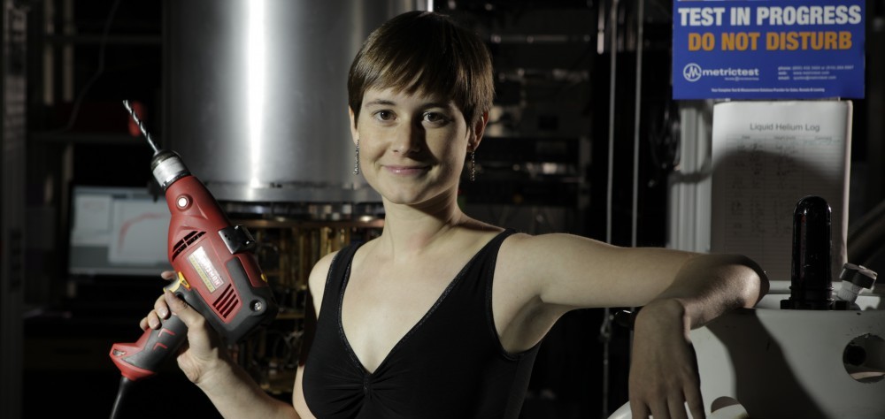
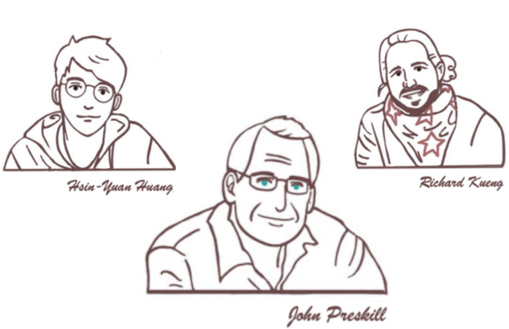


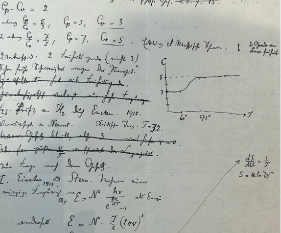
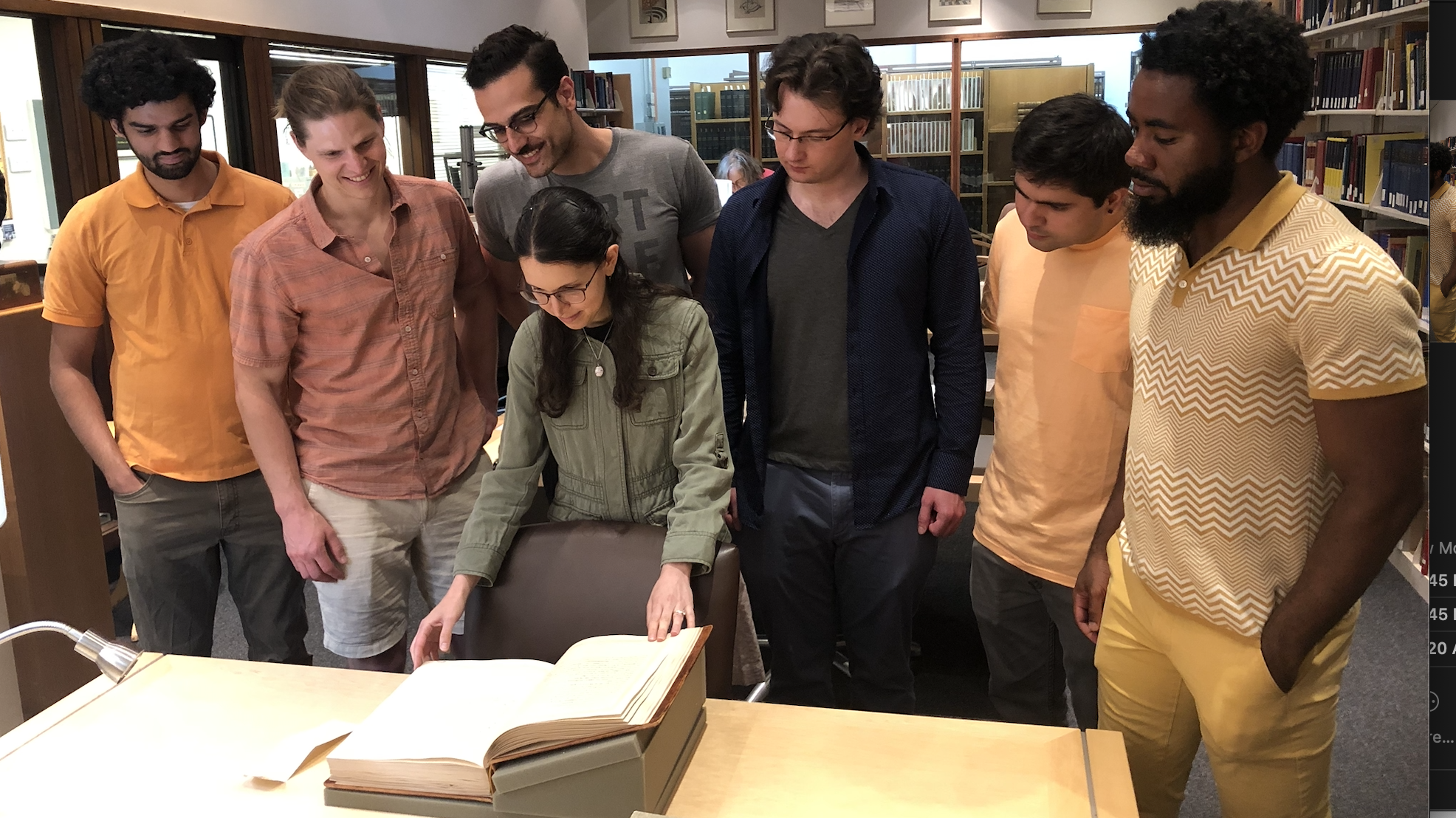

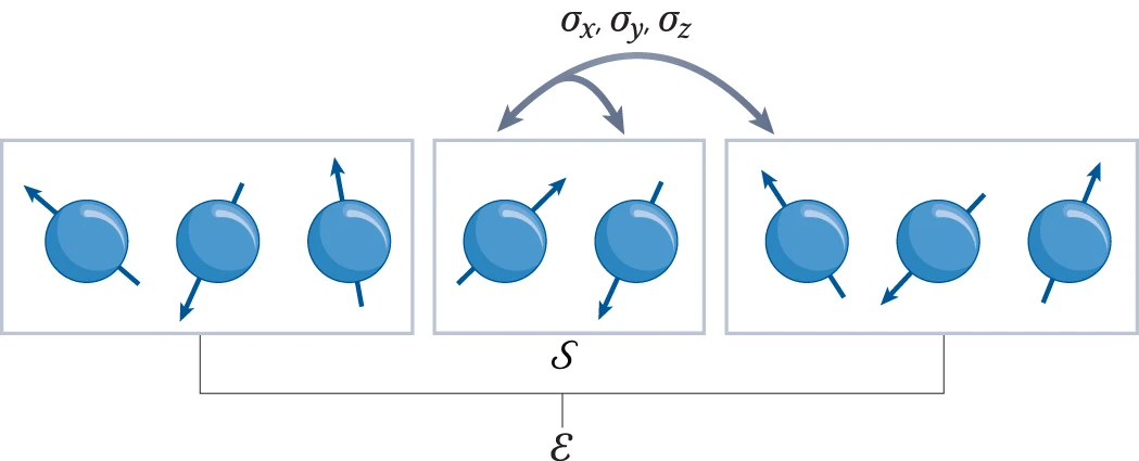
 , the “code distance”, dependent primarily on the quality of your hardware, which is somewhere in the range of 20-40. It takes
  qubits to make up a logical qubit, so let’s say 1000 of them per logical qubit. (We need to make use of an equivalent number of ancillary qubits as well). Very roughly speaking, we repeat twice the following: each physical qubit gets involved in a small number (say 4-8) of two-qubit gates with neighboring qubits, and then some subset of qubits undergo a single-qubit measurement. Most of these gates can happen simultaneously, so (again, roughly!) the time for this whole process is the time for a handful of two-qubit gates plus a measurement. It is known as a code cycle and the time it takes we denote
  . For example, in superconducting qubits this timescale is expected to be about 1 microsecond, for ion-trap qubits about 1 millisecond. Although variations exist, lets stick to considering a basic architecture which requires repeating this whole process on the order of
  , this sets the effective logical gate speed.
 , the time for a logical gate would be
  and the photonic equivalent of
  and some go into a delay of length
  .
.  that some photons spend in the longest interleaving delay line. We would like to make this as long as possible, but the maximum time is limited by the loss in the delay (typically optical fiber) and the maximum loss our error correcting code can tolerate. A number to have in mind for this (in early machines) is a handful of microseconds – corresponding to a few Km of fiber.
 . Note that this rate is distinct from any physical clock rate, as, e.g., 100 resource state generators running at 100MHz, or 10 resource state generators running at 1GHz, or 1 resource state generator running at 10GHz all yield the same total rate of resource state production

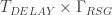 which is effectively the total number of resource states “alive” in the machine at any given instant of time, including all the ones stacked up in long delay lines. This is how we leverage optical fiber delays for a massive amplification of the entanglement our hardware has available to compute with.
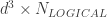 and the logical gate time of the machine is
 .
.
 microsecond code cycle – the answer is roughly that with 10 million physical superconducting qubits it would take about 4 hours (with an equivalent ion trap computer the time balloons to more than 5 months).
 1 microsecond compares to the expected
  . This could be 6000 resource state generators each producing resource states at
  or 3500 generators producing them at 1GHz for example. Then the same computation would take 58 seconds, instead of four hours, a speedup by a factor of more than 200!
 ? And what if our longest delay is ten times longer, i.e.
  microseconds (so as to be much slower than
  by building 350 billion resource state generators that can each produce resource states at only 1Hz. Yes, you read that right.
 would scale proportionally with
  and
and  . As I hope is clear by now, as a pure theoretician, I don’t give a damn if that means 10000 resource state generators running at 1MHz, 100 resource state generators running at 100MHz, or 10 resource state generators running at 1GHz. However, the fact this flexibility exists is very useful to my engineering colleagues – who, of course, aim to build the smallest and fastest possible machine they can, thereby shortening the time until we let them head off for a nice long vacation sipping mezcal margaritas on a warm tropical beach.
 . Loss reduces the rate of production considerably.


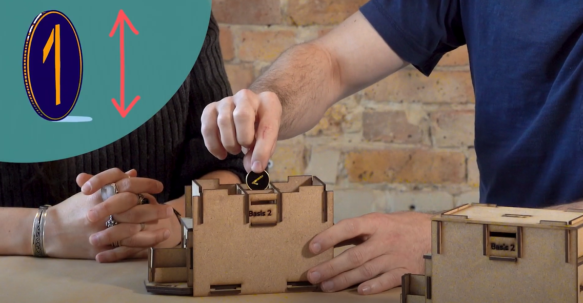


 chance that Eve got lucky and guessed Alice’s inputs correctly. To put this in perspective, a 20-round check for Eve provides a 99.9999% guarantee of security. Of course, the more rounds used to check for Eve, the fewer secure bits are left for Alice and Bob to share at the end. On average, after a total of 2(N+M) rounds, with N rounds dedicated to Eve, we get an M-bit secret key.

 eigenstate, performed a Hadamard gate, and measured
  and a 50% chance of yield
  . But the
