About Nicole Yunger Halpern

I’m a theoretical physicist at the Joint Center for Quantum Information and Computer Science in Maryland. My research group re-envisions 19th-century thermodynamics for the 21st century, using the mathematical toolkit of quantum information theory. We then apply quantum thermodynamics as a lens through which to view the rest of science. I call this research “quantum steampunk,” after the steampunk genre of art and literature that juxtaposes Victorian settings (à la thermodynamics) with futuristic technologies (à la quantum information). For more information, check out my book for the general public, Quantum Steampunk: The Physics of Yesterday’s Tomorrow. I earned my PhD at Caltech under John Preskill’s auspices; one of my life goals is to be the subject of one of his famous (if not Pullitzer-worthy) poems. Follow me on Twitter @nicoleyh11.

Gently yoking yin to yang

Posted on November 26, 2017 by Nicole Yunger Halpern

The architecture at the University of California, Berkeley mystified me. California Hall evokes a Spanish mission. The main library consists of white stone pillared by ionic columns. A sea-green building scintillates in the sunlight like a scarab. The buildings straddle the map of styles.

So do Berkeley’s quantum scientists, information-theory users, and statistical mechanics.

The chemists rove from abstract quantum information (QI) theory to experiments. Physicists experiment with superconducting qubits, trapped ions, and numerical simulations. Computer scientists invent algorithms for quantum computers to perform.

Few activities light me up more than bouncing from quantum group to info-theory group to stat-mech group, hunting commonalities. I was honored to bounce from group to group at Berkeley this September.

What a trampoline Berkeley has.

The groups fan out across campus and science, but I found compatibility. Including a collaboration that illuminated quantum incompatibility.

Quantum incompatibility originated in studies by Werner Heisenberg. He and colleagues cofounded quantum mechanics during the early 20th century. Measuring one property of a quantum system, Heisenberg intuited, can affect another property.

The most famous example involves position and momentum. Say that I hand you an electron. The electron occupies some quantum state represented by $| \Psi \rangle$ . Suppose that you measure the electron’s position. The measurement outputs one of many possible values $x$ (unless $| \Psi \rangle$ has an unusual form, the form a Dirac delta function).

But we can’t say that the electron occupies any particular point $x = x_0$ in space. Measurement devices have limited precision. You can measure the position only to within some error $\varepsilon$ : $x = x_0 \pm \varepsilon$ .

Suppose that, immediately afterward, you measure the electron’s momentum. This measurement, too, outputs one of many possible values. What probability $q(p) dp$ does the measurement have of outputting some value $p$ ? We can calculate $q(p) dp$ , knowing the mathematical form of $| \Psi \rangle$ and knowing the values of $x_0$ and $\varepsilon$ .

$q(p)$ is a probability density, which you can think of as a set of probabilities. The density can vary with $p$ . Suppose that $q(p)$ varies little: The probabilities spread evenly across the possible $p$ values. You have no idea which value your momentum measurement will output. Suppose, instead, that $q(p)$ peaks sharply at some value $p = p_0$ . You can likely predict the momentum measurement’s outcome.

The certainty about the momentum measurement trades off with the precision $\varepsilon$ of the position measurement. The smaller the $\varepsilon$ (the more precisely you measured the position), the greater the momentum’s unpredictability. We call position and momentum complementary, or incompatible.

https://www.xkcd.com/1473/

You can’t measure incompatible properties, with high precision, simultaneously. Imagine trying to do so. Upon measuring the momentum, you ascribe a tiny range of momentum values $p$ to the electron. If you measured the momentum again, an instant later, you could likely predict that measurement’s outcome: The second measurement’s $q(p)$ would peak sharply (encode high predictability). But, in the first instant, you measure also the position. Hence, by the discussion above, $q(p)$ would spread out widely. But we just concluded that $q(p)$ would peak sharply. This contradiction illustrates that you can’t measure position and momentum, precisely, at the same time.

But you can simultaneously measure incompatible properties weakly. A weak measurement has an enormous $\varepsilon$ . A weak position measurement barely spreads out $q(p)$ . If you want more details, ask a Quantum Frontiers regular; I’ve been harping on weak measurements for months.

Blame Berkeley for my harping this month. Irfan Siddiqi’s and Birgitta Whaley’s groups collaborated on weak measurements of incompatible observables. They tracked how the measured quantum state $| \Psi (t) \rangle$ evolved in time (represented by $t$ ).

Irfan’s group manipulates superconducting qubits.¹ The qubits sit in the physics building, a white-stone specimen stamped with an egg-and-dart motif. Across the street sit chemists, including members of Birgitta’s group. The experimental physicists and theoretical chemists teamed up to study a quantum lack of teaming up.

The experiment involved one superconducting qubit. The qubit has properties analogous to position and momentum: A ball, called the Bloch ball, represents the set of states that the qubit can occupy. Imagine an arrow pointing from the sphere’s center to any point in the ball. This Bloch vector represents the qubit’s state. Consider an arrow that points upward from the center to the surface. This arrow represents the qubit state $| 0 \rangle$ . $| 0 \rangle$ is the quantum analog of the possible value 0 of a bit, or unit of information. The analogous downward-pointing arrow represents the qubit state $| 1 \rangle$ , analogous to 1.

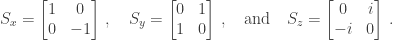
Infinitely many axes intersect the sphere. Different axes represent different observables that Irfan’s group can measure. Nonparallel axes represent incompatible observables. For example, the $x$ -axis represents an observable $\sigma_x$ analogous to position. The $y$ -axis represents an observable $\sigma_y$ analogous to momentum.

Siddiqi lab, decorated with the trademark for the paper’s tug-of-war between incompatible observables. Photo credit: Leigh Martin, one of the paper’s leading authors.

Irfan’s group stuck their superconducting qubit in a cavity, or box. The cavity contained light that interacted with the qubit. The interactions transferred information from the qubit to the light: The light measured the qubit’s state. The experimentalists controlled the interactions, controlling the axes “along which” the light was measured. The experimentalists weakly measured along two axes simultaneously.

Suppose that the axes coincided—say, at the $x$ -axis $\hat{x}$ . The qubit would collapse to the state $| \Psi \rangle = \frac{1}{ \sqrt{2} } ( | 0 \rangle + | 1 \rangle )$ , represented by the arrow that points along $\hat{x}$ to the sphere’s surface, or to the state $| \Psi \rangle = \frac{1}{ \sqrt{2} } ( | 0 \rangle - | 1 \rangle )$ , represented by the opposite arrow.

(Projection of) the Bloch Ball after the measurement. The system can access the colored points. The lighter a point, the greater the late-time state’s weight on the point.

Let $\hat{x}'$ denote an axis near $\hat{x}$ —say, 18° away. Suppose that the group weakly measured along $\hat{x}$ and $\hat{x}'$ . The state would partially collapse. The system would access points in the region straddled by $\hat{x}$ and $\hat{x}'$ , as well as points straddled by $- \hat{x}$ and $- \hat{x}'$ .

Finally, suppose that the group weakly measured along $\hat{x}$ and $\hat{y}$ . These axes stand in for position and momentum. The state would, loosely speaking, swirl around the Bloch ball.

The Berkeley experiment illuminates foundations of quantum theory. Incompatible observables, physics students learn, can’t be measured simultaneously. This experiment blasts our expectations, using weak measurements. But the experiment doesn’t just destroy. It rebuilds the blast zone, by showing how $| \Psi (t) \rangle$ evolves.

“Position” and “momentum” can hang together. So can experimentalists and theorists, physicists and chemists. So, somehow, can the California mission and the ionic columns. Maybe I’ll understand the scarab building when we understand quantum theory.²

With thanks to Birgitta’s group, Irfan’s group, and the rest of Berkeley’s quantum/stat-mech/info-theory community for its hospitality. The Bloch-sphere figures come from http://www.nature.com/articles/nature19762.

¹The qubit is the quantum analog of a bit. The bit is the basic unit of information. A bit can be in one of two possible states, which we can label as 0 and 1. Qubits can manifest in many physical systems, including superconducting circuits. Such circuits are tiny quantum circuits through which current can flow, without resistance, forever.

²Soda Hall dazzled but startled me.

Paradise

Posted on October 22, 2017 by Nicole Yunger Halpern

The word dominates chapter one of Richard Holmes’s book The Age of Wonder. Holmes writes biographies of Romantic-Era writers: Mary Wollstonecraft, Percy Shelley, and Samuel Taylor Coleridge populate his bibliography. They have cameos in Age. But their scientific counterparts star.

“Their natural-philosopher” counterparts, I should say. The word “scientist” emerged as the Romantic Era closed. Romanticism, a literary and artistic movement, flourished between the 1700s and the 1800s. Romantics championed self-expression, individuality, and emotion over convention and artificiality. Romantics wondered at, and drew inspiration from, the natural world. So, Holmes argues, did Romantic-Era natural philosophers. They explored, searched, and innovated with Wollstonecraft’s, Shelley’s, and Coleridge’s zest.

Holmes depicts Wilhelm and Caroline Herschel, a German brother and sister, discovering the planet Uranus. Humphry Davy, an amateur poet from Penzance, inventing a lamp that saved miners’ lives. Michael Faraday, a working-class Londoner, inspired by Davy’s chemistry lectures.

Joseph Banks in paradise.

So Holmes entitled chapter one.

Banks studied natural history as a young English gentleman during the 1760s. He then sailed around the world, a botanist on exploratory expeditions. The second expedition brought Banks aboard the HMS Endeavor. Captain James Cook steered the ship to Brazil, Tahiti, Australia, and New Zealand. Banks brought a few colleagues onboard. They studied the native flora, fauna, skies, and tribes.

Banks, with fellow botanist Daniel Solander, accumulated over 30,000 plant samples. Artist Sydney Parkinson drew the plants during the voyage. Parkinson’s drawings underlay 743 copper engravings that Banks commissioned upon returning to England. Banks planned to publish the engravings as the book Florilegium. He never succeeded. Two institutions executed Banks’s plan more than 200 years later.

Banks’s Florilegium crowns an exhibition at the University of California at Santa Barbara (UCSB). UCSB’s Special Research Collections will host “Botanical Illustrations and Scientific Discovery—Joseph Banks and the Exploration of the South Pacific, 1768–1771” until May 2018. The exhibition features maps of Banks’s journeys, biographical sketches of Banks and Cook, contemporary art inspired by the engravings, and the Florilegium.

The exhibition spotlights “plants that have subsequently become important ornamental plants on the UCSB campus, throughout Santa Barbara, and beyond.” One sees, roaming Santa Barbara, slivers of Banks’s paradise.

In Santa Barbara resides the Kavli Institute for Theoretical Physics (KITP). The KITP is hosting a program about the physics of quantum information (QI). QI scientists are congregating from across the world. Everyone visits for a few weeks or months, meeting some participants and missing others (those who have left or will arrive later). Participants attend and present tutorials, explore beyond their areas of expertise, and initiate research collaborations.

A conference capstoned the program, one week this October. Several speakers had founded subfields of physics: quantum error correction (how to fix errors that dog quantum computers), quantum computational complexity (how quickly quantum computers can solve hard problems), topological quantum computation, AdS/CFT (a parallel between certain gravitational systems and certain quantum systems), and more. Swaths of science exist because of these thinkers.

One evening that week, I visited the Joseph Banks exhibition.

Joseph Banks in paradise.

I’d thought that, by “paradise,” Holmes had meant “physical attractions”: lush flowers, vibrant colors, fresh fish, and warm sand. Another meaning occurred to me, after the conference talks, as I stood before a glass case in the library.

Joseph Banks, disembarking from the Endeavour, didn’t disembark onto just an island. He disembarked onto terra incognita. Never had he or his colleagues seen the blossoms, seed pods, or sprouts before him. Swaths of science awaited. What could the natural philosopher have craved more?

QI scientists of a certain age reminisce about the 1990s, the cowboy days of QI. When impactful theorems, protocols, and experiments abounded. When they dangled, like ripe fruit, just above your head. All you had to do was look up, reach out, and prove a pineapple.

Typical 1990s quantum-information scientist

That generation left mine few simple theorems to prove. But QI hasn’t suffered extinction. Its frontiers have advanced into other fields of science. Researchers are gaining insight into thermodynamics, quantum gravity, condensed matter, and chemistry from QI. The KITP conference highlighted connections with quantum gravity.

…in paradise.

What could a natural philosopher crave more?

Artwork commissioned by the UCSB library: “Sprawling Neobiotic Chimera (After Banks’ Florilegium),” by Rose Briccetti

Most KITP talks are recorded and released online. You can access talks from the conference here. My talk, about quantum chaos and thermalization, appears here.

With gratitude to the KITP, and to the program organizers and the conference organizers, for the opportunity to participate.

Standing back at Stanford

Posted on September 17, 2017 by Nicole Yunger Halpern

This T-shirt came to mind last September. I was standing in front of a large silver-colored table littered with wires, cylinders, and tubes. Greg Bentsen was pointing at components and explaining their functions. He works in Monika Schleier-Smith’s lab, as a PhD student, at Stanford.

Monika’s group manipulates rubidium atoms. A few thousand atoms sit in one of the cylinders. That cylinder contains another cylinder, an optical cavity, that contains the atoms. A mirror caps each of the cavity’s ends. Light in the cavity bounces off the mirrors.

Light bounces off your bathroom mirror similarly. But we can describe your bathroom’s light accurately with Maxwellian electrodynamics, a theory developed during the 1800s. We describe the cavity’s light with quantum electrodynamics (QED). Hence we call the lab’s set-up cavity QED.

The light interacts with the atoms, entangling with them. The entanglement imprints information about the atoms on the light. Suppose that light escaped from the cavity. Greg and friends could measure the light, then infer about the atoms’ quantum state.

A little light leaks through the mirrors, though most light bounces off. From leaked light, you can infer about the ensemble of atoms. You can’t infer about individual atoms. For example, consider an atom’s electrons. Each electron has a quantum property called a spin. We sometimes imagine the spin as an arrow that points upward or downward. Together, the electrons’ spins form the atom’s joint spin. You can tell, from leaked light, whether one atom’s spin points upward. But you can’t tell which atom’s spin points upward. You can’t see the atoms for the ensemble.

Monika’s team can. They’ve cut a hole in their cylinder. Light escapes the cavity through the hole. The light from the hole’s left-hand edge carries information about the leftmost atom, and so on. The team develops a photograph of the line of atoms. Imagine holding a photograph of a line of people. You can point to one person, and say, “Aha! She’s the xkcd fan.” Similarly, Greg and friends can point to one atom in their photograph and say, “Aha! That atom has an upward-pointing spin.” Monika’s team is developing single-site imaging.

Aha! She’s the xkcd fan.

Monika’s team plans to image atoms in such detail, they won’t need for light to leak through the mirrors. Light leakage creates problems, including by entangling the atoms with the world outside the cavity. Suppose you had to diminish the amount of light that leaks from a rubidium cavity. How should you proceed?

Tell the mirrors,

You should lengthen the cavity. Why? Imagine a photon, a particle of light, in the cavity. It zooms down the cavity’s length, hits a mirror, bounces off, retreats up the cavity’s length, hits the other mirror, and bounces off. The photon repeats this process until a mirror hit fails to generate a bounce. The mirror transmits the photon to the exterior; the photon leaks out. How can you reduce leaks? By preventing photons from hitting mirrors so often, by forcing the photons to zoom longer, by lengthening the cavity, by shifting the mirrors outward.

So Greg hinted, beside that silver-colored table in Monika’s lab. The hint struck a chord: I recognized the impulse to

The impulse had led me to Stanford.

Weeks earlier, I’d written my first paper about quantum chaos and information scrambling. I’d sat and read and calculated and read and sat and emailed and written. I needed to stand up, leave my cavity, and image my work from other perspectives.

Stanford physicists had written quantum-chaos papers I admired. So I visited, presented about my work, and talked. Patrick Hayden introduced me to a result that might help me apply my result to another problem. His group helped me simplify a mathematical expression. Monika reflected that a measurement scheme I’d proposed sounded not unreasonable for cavity QED.

And Greg led me to recognize the principle behind my visit: Sometimes, you have to

to move forward.

With gratitude to Greg, Monika, Patrick, and the rest of Monika’s and Patrick’s groups for their time, consideration, explanations, and feedback. With thanks to Patrick and Stanford’s Institute for Theoretical Physics for their hospitality.

Decoding (the allure of) the apparent horizon

Posted on August 27, 2017 by Nicole Yunger Halpern

I took 32 hours to unravel why Netta Engelhardt’s talk had struck me.

We were participating in Quantum Information in Quantum Gravity III, a workshop hosted by the University of British Columbia (UBC) in Vancouver. Netta studies quantum gravity as a Princeton postdoc. She discussed a feature of black holes—an apparent horizon—I’d not heard of. After hearing of it, I had to grasp it. I peppered Netta with questions three times in the following day. I didn’t understand why, for 32 hours.

After 26 hours, I understood apparent horizons like so.

Imagine standing beside a glass sphere, an empty round shell. Imagine light radiating from a point source in the sphere’s center. Think of the point source as a minuscule flash light. Light rays spill from the point source.

Which paths do the rays follow through space? They fan outward from the sphere’s center, hit the glass, and fan out more. Imagine turning your back to the sphere and looking outward. Light rays diverge as they pass you.

At least, rays diverge in flat space-time. We live in nearly flat space-time. We wouldn’t if we neighbored a supermassive object, like a black hole. Mass curves space-time, as described by Einstein’s theory of general relativity.

Imagine standing beside the sphere near a black hole. Let the sphere have roughly the black hole’s diameter—around 10 kilometers, according to astrophysical observations. You can’t see much of the sphere. So—imagine—you recruit your high-school-physics classmates. You array yourselves around the sphere, planning to observe light and compare observations. Imagine turning your back to the sphere. Light rays would converge, or flow toward each other. You’d know yourself to be far from Kansas.

Picture you, your classmates, and the sphere falling into the black hole. When would everyone agree that the rays switch from diverging to converging? Sometime after you passed the event horizon, the point of no return.¹ Before you reached the singularity, the black hole’s center, where space-time warps infinitely. The rays would switch when you reached an in-between region, the apparent horizon.

Imagine pausing at the apparent horizon with your sphere, facing away from the sphere. Light rays would neither diverge nor converge; they’d point straight. Continue toward the singularity, and the rays would converge. Reverse away from the singularity, and the rays would diverge.

UBC near twilight

Rays diverged from the horizon beyond UBC at twilight. Twilight suits UBC as marble suits the Parthenon; and UBC’s twilight suits musing. You can reflect while gazing on reflections in glass buildings, or reflections in a pool by a rose garden. Your mind can roam as you roam paths lined by elms, oaks, and willows. I wandered while wondering why the sphere intrigued me.

Science thrives on instrumentation. Galileo improved the telescope, which unveiled Jupiter’s moons. Alexander von Humboldt measured temperatures and pressures with thermometers and barometers, charting South America during the 1700s. The Large Hadron Collider revealed the Higgs particle’s mass in 2012.

The sphere reminded me of a thermometer. As thermometers register temperature, so does the sphere register space-time curvature. Not that you’d need a sphere to distinguish a black hole from Kansas. Nor do you need a thermometer to distinguish Vancouver from a Brazilian jungle. But thermometers quantify the distinction. A sphere would sharpen your observations’ precision.

A sphere and a light source—free of supercolliders, superconductors, and superfridges. The instrument boasts not only profundity, but also simplicity.

Alexander von Humboldt

Netta proved a profound theorem about apparent horizons, with coauthor Aron Wall. Jakob Bekenstein and Stephen Hawking had studied event horizons during the 1970s. An event horizon’s area, Bekenstein and Hawking showed, is proportional to the black hole’s thermodynamic entropy. Netta and Aron proved a proportionality between another area and another entropy.

They calculated an apparent horizon’s area, $A$ . The math that represents their black hole represents also a quantum system, by a duality called AdS/CFT. The quantum system can occupy any of several states. Different states encode different information about the black hole. Consider the information needed to describe, fully and only, the region outside the apparent horizon. Some quantum state $\rho$ encodes this information. $\rho$ encodes no information about the region behind the apparent horizon, closer to the black hole. How would you quantify this lack of information? With the von Neumann entropy $S(\rho)$ . This entropy is proportional to the apparent horizon’s area: $S( \rho ) \propto A$ .

Netta and Aron entitled their paper “Decoding the apparent horizon.” Decoding the apparent horizon’s allure took me 32 hours and took me to an edge of campus. But I didn’t mind. Edges and horizons suited my visit as twilight suits UBC. Where can we learn, if not at edges, as where quantum information meets other fields?

With gratitude to Mark van Raamsdonk and UBC for hosting Quantum Information in Quantum Gravity III; to Mark, the other organizers, and the “It from Qubit” Simons Foundation collaboration for the opportunity to participate; and to Netta Engelhardt for sharing her expertise.

¹Nothing that draws closer to a black hole than the event horizon can turn around and leave, according to general relativity. The black hole’s gravity pulls too strongly. Quantum mechanics implies that information leaves, though, in Hawking radiation.

The sign problem(s)

Posted on July 27, 2017 by Nicole Yunger Halpern

The thirteen-month-old had mastered the word “dada” by the time I met her. Her parents were teaching her to communicate other concepts through sign language. Picture her, dark-haired and bibbed, in a high chair. Banana and mango slices litter the tray in front of her. More fruit litters the floor in front of the tray. The baby lifts her arms and flaps her hands.

Dada looks up from scrubbing the floor.

“Look,” he calls to Mummy, “she’s using sign language! All done.” He performs the gesture that his daughter seems to have aped: He raises his hands and rotates his forearms about his ulnas, axes perpendicular to the floor. “All done!”

The baby looks down, seizes another morsel, and stuffs it into her mouth.

“Never mind,” Dada amends. “You’re not done, are you?”

His daughter had a sign(-language) problem.

So does Dada, MIT professor Aram Harrow. Aram studies quantum information theory. His interests range from complexity to matrices, from resource theories to entropies. He’s blogged for The Quantum Pontiff, and he studies—including with IQIM postdoc Elizabeth Crosson—the quantum sign problem.

Imagine calculating properties of a chunk of fermionic quantum matter. The chunk consists of sites, each inhabited by one particle or by none. Translate as “no site can house more than one particle” the jargon “the particles are fermions.”

The chunk can have certain amounts of energy. Each amount $E_j$ corresponds to some particle configuration indexed by $j$ : If the system has some amount $E_1$ of energy, particles occupy certain sites and might not occupy others. If the system has a different amount $E_2 \neq E_1$ of energy, particles occupy different sites. A Hamiltonian, a mathematical object denoted by $H,$ encodes the energies $E_j$ and the configurations. We represent $H$ with a matrix, a square grid of numbers.

Suppose that the chunk has a temperature $T = \frac{ 1 }{ k_{\rm B} \beta }$ . We could calculate the system’s heat capacity, the energy required to raise the chunk’s temperature by one Kelvin. We could calculate the free energy, how much work the chunk could perform in powering a motor or lifting a weight. To calculate those properties, we calculate the system’s partition function, $Z$ .

How? We would list the configurations $j$ . With each configuration, we would associate the weight $e^{ - \beta E_j }$ . We would sum the weights: $Z = e^{ - \beta E_1 } + e^{ - \beta E_2} + \ldots = \sum_j e^{ - \beta E_j}$ .

Easier—like feeding a 13-month-old—said than done. Let $N$ denote the number of qubits in the chunk. If $N$ is large, the number of configurations is gigantic. Our computers can’t process so many configurations. This inability underlies quantum computing’s promise of speeding up certain calculations.

We don’t have quantum computers, and we can’t calculate $Z$ . Can we approximate $Z$ ?

Yes, if $H$ “lacks the sign problem.” The math that models our system models also a classical system. If our system has $D$ dimensions, the classical system has $D+1$ dimensions. Suppose, for example, that our sites form a line. The classical system forms a square.

We replace the weights $e^{ - \beta E_j }$ with different weights—numbers formed from a matrix that represents $H$ . If $H$ lacks the sign problem, the new weights are nonnegative and behave like probabilities. Many mathematical tools suit probabilities. Aram and Elizabeth apply such tools to $Z$ , here and here, as do many other researchers.

We call Hamiltonians that lack the sign problem “stoquastic,” which I think fanquastic.¹Stay tuned for a blog post about stoquasticity by Elizabeth.

What if $H$ has the sign problem? The new weights can assume negative and nonreal values. The weights behave unlike probabilities; we can’t apply those tools. We find ourselves knee-deep in banana and mango chunks.

Solutions to the sign problem remain elusive. Theorists keep trying to mitigate the problem, though. Aram, Elizabeth, and others are improving calculations of properties of sign-problem-free systems. One scientist-in-the-making has achieved a breakthrough: Aram’s daughter now rotates her hands upon finishing meals and when she wants to leave her car seat or stroller.

One sign problem down; one to go.

With gratitude to Aram’s family for its hospitality and to Elizabeth Crosson for sharing her expertise.

¹For experts: A local Hamiltonian is stoquastic relative to the computational basis if each local term is represented, relative to the computational basis, by a matrix whose off-diagonal entries are real and nonpositive.

Time capsule at the Dibner Library

Posted on June 18, 2017 by Nicole Yunger Halpern

The first time I met Lilla Vekerdy, she was holding a book.

“What’s that?” I asked.

“A second edition of Galileo’s Siderius nuncius. Here,” she added, thrusting the book into my hands. “Take it.”

So began my internship at the Smithsonian Institution’s Dibner Library for the History of Science and Technology.

Many people know the Smithsonian for its museums. The Smithsonian, they know, houses the ruby slippers worn by Dorothy in The Wizard of Oz. The Smithsonian houses planes constructed by Orville and Wilbur Wright, the dresses worn by First Ladies on presidential inauguration evenings, a space shuttle, and a Tyrannosaurus Rex skeleton. Smithsonian museums line the National Mall in Washington, D.C.—the United States’ front lawn—and march beyond.

Most people don’t know that the Smithsonian has 21 libraries.

Lilla heads the Smithsonian Libraries’ Special-Collections Department. She also directs a library tucked into a corner of the National Museum of American History. I interned at that library—the Dibner—in college. Images of Benjamin Franklin, of inventor Eli Whitney, and of astronomical instruments line the walls. The reading room contains styrofoam cushions on which scholars lay crumbling rare books. Lilla and the library’s technician, Morgan Aronson, find references for researchers, curate exhibitions, and introduce students to science history. They also care for the vault.

The vault. How I’d missed the vault.

A corner of the Dibner’s reading room and part of the vault

The vault contains manuscripts and books from the past ten centuries. We handle the items without gloves, which reduce our fingers’ sensitivities: Interpose gloves between yourself and a book, and you’ll raise your likelihood of ripping a page. A temperature of 65°F inhibits mold from growing. Redrot mars some leather bindings, though, and many crowns—tops of books’ spines—have collapsed. Aging carries hazards.

But what the ages have carried to the Dibner! We¹ have a survey filled out by Einstein and a first edition of Newton’s Principia mathematica. We have Euclid’s Geometry in Latin, Arabic, and English, from between 1482 and 1847. We have a note, handwritten by quantum physicist Erwin Schödinger, about why students shouldn’t fear exams.

I returned to the Dibner one day this spring. Lilla and I fetched out manuscripts and books related to quantum physics and thermodynamics. “Hermann Weyl” labeled one folder.

Weyl contributed to physics and mathematics during the early 1900s. I first encountered his name when studying particle physics. The Dibner, we discovered, owns a proof for part of his 1928 book Gruppentheorie und Quantenmechanik. Weyl appears to have corrected a typed proof by hand. He’d handwritten also spin matrices.

Electrons have a property called “spin.” Spin resembles a property of yours, your position relative to the Earth’s center. We represent your position with three numbers: your latitude, your longitude, and your distance above the Earth’s surface. We represent electron spin with three blocks of numbers, three $2 \times 2$ matrices. Today’s physicists write the matrices as²

$S_x = \begin{bmatrix} 0 & 1 \\ 1 & 0 \end{bmatrix} \, , \quad S_y = \begin{bmatrix} 0 & -i \\ i & 0 \end{bmatrix} \, , \quad \text{and} \quad S_z = \begin{bmatrix} -1 & 0 \\ 0 & 1 \end{bmatrix} \, .$

We needn’t write these matrices. We could represent electron spin with different $2 \times 2$ matrices, so long as the matrices obey certain properties. But most physicists choose the above matrices, in my experience. We call our choice “a convention.”

Weyl chose a different convention:

$S_x = \begin{bmatrix} 1 & 0 \\ 0 & -1 \end{bmatrix} \, , \quad S_y = \begin{bmatrix} 0 & 1 \\ 1 & 0 \end{bmatrix} \, , \quad \text{and} \quad S_z = \begin{bmatrix} 0 & i \\ -i & 0 \end{bmatrix} \, .$

The difference surprised me. Perhaps it shouldn’t have: Conventions change. Approaches to quantum physics change. Weyl’s matrices differ from ours little: Permute our matrices and negate one matrix, and you recover Weyl’s.

But the electron-spin matrices play a role, in quantum physics, like the role played by T. Rex in paleontology exhibits: All quantum scientists recognize electron spin. We illustrate with electron spin in examples. Students memorize spin matrices in undergrad classes. Homework problems feature electron spin. Physicists have known of electron spin’s importance for decades. I didn’t expect such a bedrock to have changed its trappings.

How did scientists’ convention change? When did it? Why? Or did the convention not change—did Weyl’s contemporaries use today’s convention, and did Weyl stand out?

A partially typed, partially handwritten, proof of a book by Hermann Weyl.

I intended to end this article with these questions. I sent a draft to John Preskill, proposing to post soon. But he took up the questions like a knight taking up arms.

Wolfgang Pauli, John emailed, appears to have written the matrices first. (Physicist call the matrices “Pauli matrices.”) A 1927 paper by Pauli contains the notation used today. Paul Dirac copied the notation in a 1928 paper, acknowledging Pauli. Weyl’s book appeared the same year. The following year, Weyl used Pauli’s notation in a paper.

No document we know of, apart from the Dibner proof, contains the Dibner-proof notation. Did the notation change between the proof-writing and publication? Does the Dibner hold the only anomalous electron-spin matrices? What accounts for the anomaly?

If you know, feel free to share. If you visit DC, drop Lilla and Morgan a line. Bring a research project. Bring a class. Bring zeal for the past. You might find yourself holding a time capsule by Galileo.

Dibner librarian Lilla Vekerdy and a former intern

With thanks to Lilla and Morgan for their hospitality, time, curiosity, and expertise. With thanks to John for burrowing into the Pauli matrices’ history.

¹I continue to count myself as part of the Dibner community. Part of me refuses to leave.

²I’ll omit factors of $\hbar / 2 \, .$

The power of information

Posted on May 21, 2017 by Nicole Yunger Halpern

Sara Imari Walker studies ants. Her entomologist colleague Gabriele Valentini cultivates ant swarms. Gabriele coaxes a swarm from its nest, hides the nest, and offers two alternative nests. Gabriele observe the ants’ responses, then analyzes their data with Sara.

Sara doesn’t usually study ants. She trained in physics, information theory, and astrobiology. (Astrobiology is the study of life; life’s origins; and conditions amenable to life, on Earth and anywhere else life may exist.) Sara analyzes how information reaches, propagates through, and manifests in the swarm.

Some ants inspect one nest; some, the other. Few ants encounter both choices. Yet most of the ants choose simultaneously. (How does Gabriele know when an ant chooses? Decided ants carry other ants toward the chosen nest. Undecided ants don’t.)

Gabriele and Sara plotted each ant’s status (decided or undecided) at each instant. All the ants’ lines start in the “undecided” region, high up in the graph. Most lines drop to the “decided” region together. Physicists call such dramatic, large-scale changes in many-particle systems “phase transitions.” The swarm transitions from the “undecided” phase to the “decided,” as moisture transitions from vapor to downpour.

Sara versus the ants

Look from afar, and you’ll see evidence of a hive mind: The lines clump and slump together. Look more closely, and you’ll find lags between ants’ decisions. Gabriele and Sara grouped the ants according to their behaviors. Sara explained the grouping at a workshop this spring.

The green lines, she said, are undecided ants.

My stomach dropped like Gabriele and Sara’s ant lines.

People call data “cold” and “hard.” Critics lambast scientists for not appealing to emotions. Politicians weave anecdotes into their numbers, to convince audiences to care.

But when Sara spoke, I looked at her green lines and thought, “That’s me.”

I’ve blogged about my indecisiveness. Postdoc Ning Bao and I formulated a quantum voting scheme in which voters can superpose—form quantum combinations of—options. Usually, when John Preskill polls our research group, I abstain from voting. Politics, and questions like “Does building a quantum computer require only engineering or also science?”,¹ have many facets. I want to view such questions from many angles, to pace around the questions as around a sculpture, to hear other onlookers, to test my impressions on them, and to cogitate before choosing.² However many perspectives I’ve gathered, I’m missing others worth seeing. I commiserated with the green-line ants.

I first met Sara in the building behind the statue. Sara earned her PhD in Dartmouth College’s physics department, with Professor Marcelo Gleiser.

Sara presented about ants at a workshop hosted by the Beyond Center for Fundamental Concepts in Science at Arizona State University (ASU). The organizers, Paul Davies of Beyond and Andrew Briggs of Oxford, entitled the workshop “The Power of Information.” Participants represented information theory, thermodynamics and statistical mechanics, biology, and philosophy.

Paul and Andrew posed questions to guide us: What status does information have? Is information “a real thing” “out there in the world”? Or is information only a mental construct? What roles can information play in causation?

We paced around these questions as around a Chinese viewing stone. We sat on a bench in front of those questions, stared, debated, and cogitated. We taught each other about ants, artificial atoms, nanoscale machines, and models for information processing.

Chinese viewing stone in Yuyuan Garden in Shanghai

I wonder if I’ll acquire opinions about Paul and Andrew’s questions. Maybe I’ll meander from “undecided” to “decided” over a career. Maybe I’ll phase-transition like Sara’s ants. Maybe I’ll remain near the top of her diagram, a green holdout.

I know little about information’s power. But Sara’s plot revealed one power of information: Information can move us—from homeless to belonging, from ambivalent to decided, from a plot’s top to its bottom, from passive listener to finding yourself in a green curve.

With thanks to Sara Imari Walker, Paul Davies, Andrew Briggs, Katherine Smith, and the Beyond Center for their hospitality and thoughts.

¹By “only engineering,” I mean not “merely engineering” pejoratively, but “engineering and no other discipline.”

²I feel compelled to perform these activities before choosing. I try to. Psychological experiments, however, suggest that I might decide before realizing that I’ve decided.

Glass beads and weak-measurement schemes

Posted on April 23, 2017 by Nicole Yunger Halpern

Richard Feynman fiddled with electronics in a home laboratory, growing up. I fiddled with arts and crafts.¹ I glued popsicle sticks, painted plaques, braided yarn, and designed greeting cards. Of the supplies in my family’s crafts box, I adored the beads most. Of the beads, I favored the glass ones.

I would pour them on the carpet, some weekend afternoons. I’d inherited a hodgepodge: The beads’ sizes, colors, shapes, trimmings, and craftsmanship varied. No property divided the beads into families whose members looked like they belonged together. But divide the beads I tried. I might classify them by color, then subdivide classes by shape. The color and shape groupings precluded me from grouping by size. But, by loosening my original classification and combining members from two classes, I might incorporate trimmings into the categorization. I’d push my classification scheme as far as I could. Then, I’d rake the beads together and reorganize them according to different principles.

Why have I pursued theoretical physics? many people ask. I have many answers. They include “Because I adored organizing craft supplies at age eight.” I craft and organize ideas.

I’ve blogged about the out-of-time-ordered correlator (OTOC), a signature of how quantum information spreads throughout a many-particle system. Experimentalists want to measure the OTOC, to learn how information spreads. But measuring the OTOC requires tight control over many quantum particles.

I proposed a scheme for measuring the OTOC, with help from Chapman University physicist Justin Dressel. The scheme involves weak measurements. Weak measurements barely disturb the systems measured. (Most measurements of quantum systems disturb the measured systems. So intuited Werner Heisenberg when formulating his uncertainty principle.)

I had little hope for the weak-measurement scheme’s practicality. Consider the stereotypical experimentalist’s response to a stereotypical experimental proposal by a theorist: Oh, sure, we can implement that—in thirty years. Maybe. If the pace of technological development doubles. I expected to file the weak-measurement proposal in the “unfeasible” category.

But experimentalists started collaring me. The scheme sounds reasonable, they said. How many trials would one have to perform? Did the proposal require ancillas, helper systems used to control the measured system? Must each ancilla influence the whole measured system, or could an ancilla interact with just one particle? How did this proposal compare with alternatives?

I met with a cavity-QED² experimentalist and a cold-atoms expert. I talked with postdocs over skype, with heads of labs at Caltech, with grad students in Taiwan, and with John Preskill in his office. I questioned an NMR³ experimentalist over lunch and fielded superconducting-qubit⁴ questions in the sunshine. I read papers, reread papers, and powwowed with Justin.

I wouldn’t have managed half so well without Justin and without Brian Swingle. Brian and coauthors proposed the first OTOC-measurement scheme. He reached out after finding my first OTOC paper.

According to that paper, the OTOC is a moment of a quasiprobability.⁵ How does that quasiprobability look, we wondered? How does it behave? What properties does it have? Our answers appear in a paper we released with Justin this month. We calculate the quasiprobability in two examples, prove properties of the quasiprobability, and argue that the OTOC motivates generalizations of quasiprobability theory. We also enhance the weak-measurement scheme and analyze it.

Amidst that analysis, in a 10 x 6 table, we classify glass beads.

We inventoried our experimental conversations and distilled them. We culled measurement-scheme features analogous to bead size, color, and shape. Each property labels a row in the table. Each measurement scheme labels a column. Each scheme has, I learned, gold flecks and dents, hues and mottling, an angle at which it catches the light.

I’ve kept most of the glass beads that fascinated me at age eight. Some of the beads have dispersed to necklaces, picture frames, and eyeglass leashes. I moved the remnants, a few years ago, to a compartmentalized box. Doesn’t it resemble the table?

That’s why I work at the IQIM.

¹I fiddled in a home laboratory, too, in a garage. But I lived across the street from that garage. I lived two rooms from an arts-and-crafts box.

²Cavity QED consists of light interacting with atoms in a box.

³Lots of nuclei manipulated with magnetic fields. “NMR” stands for “nuclear magnetic resonance.” MRI machines, used to scan brains, rely on NMR.

⁴Superconducting circuits are tiny, cold quantum circuits.

⁵A quasiprobability resembles a probability but behaves more oddly: Probabilities range between zero and one; quasiprobabilities can dip below zero. Think of a moment as like an average.

With thanks to all who questioned me; to all who answered questions of mine; to my wonderful coauthors; and to my parents, who stocked the crafts box.

Local operations and Chinese communications

Posted on March 19, 2017 by Nicole Yunger Halpern

The workshop spotlighted entanglement. It began in Shanghai, paused as participants hopped the Taiwan Strait, and resumed in Taipei. We discussed quantum operations and chaos, thermodynamics and field theory.¹ I planned to return from Taipei to Shanghai to Los Angeles.

Quantum thermodynamicist Nelly Ng and I drove to the Taipei airport early. News from Air China curtailed our self-congratulations: China’s military was running an operation near Shanghai. Commercial planes couldn’t land. I’d miss my flight to LA.

Two quantum thermodynamicists in Shanghai

An operation?

Quantum information theorists use a mindset called operationalism. We envision experimentalists in separate labs. Call the experimentalists Alice, Bob, and Eve (ABE). We tell stories about ABE to formulate and analyze problems. Which quantum states do ABE prepare? How do ABE evolve, or manipulate, the states? Which measurements do ABE perform? Do they communicate about the measurements’ outcomes?

Operationalism concretizes ideas. The outlook checks us from drifting into philosophy and into abstractions difficult to apply physics tools to.² Operationalism infuses our language, our framing of problems, and our mathematical proofs.

Experimentalists can perform some operations more easily than others. Suppose that Alice controls the magnets, lasers, and photodetectors in her lab; Bob controls the equipment in his; and Eve controls the equipment in hers. Each experimentalist can perform local operations (LO). Suppose that Alice, Bob, and Eve can talk on the phone and send emails. They exchange classical communications (CC).

You can’t generate entanglement using LOCC. Entanglement consists of strong correlations that quantum systems can share and that classical systems can’t. A quantum system in Alice’s lab can hold more information about a quantum system of Bob’s than any classical system could. We must create and control entanglement to operate quantum computers. Creating and controlling entanglement poses challenges. Hence quantum information scientists often model easy-to-perform operations with LOCC.

Suppose that some experimentalist Charlie loans entangled quantum systems to Alice, Bob, and Eve. How efficiently can ABE compute some quantity, exchange quantum messages, or perform other information-processing tasks, using that entanglement? Such questions underlie quantum information theory.

Taipei’s night market. Or Caltech’s neighborhood?

Local operations.

Nelly and I performed those, trying to finagle me to LA. I inquired at Air China’s check-in desk in English. Nelly inquired in Mandarin. An employee smiled sadly at each of us.

We branched out into classical communications. I called Expedia (“No, I do not want to fly to Manila”), United Airlines (“No flights for two days?”), my credit-card company, Air China’s American reservations office, Air China’s Chinese reservations office, and Air China’s Taipei reservations office. I called AT&T to ascertain why I couldn’t reach Air China (“Yes, please connect me to the airline. Could you tell me the number first? I’ll need to dial it after you connect me and the call is then dropped”).

As I called, Nelly emailed. She alerted Bob, aka Janet (Ling-Yan) Hung, who hosted half the workshop at Fudan University in Shanghai. Nelly emailed Eve, aka Feng-Li Lin, who hosted half the workshop at National Taiwan University in Taipei. Janet twiddled the magnets in her lab (investigated travel funding), and Feng-Li cooled a refrigerator in his.

ABE can process information only so efficiently, using LOCC. The time crept from 1:00 PM to 3:30.

Nelly Ng uses classical communications.

What could we have accomplished with quantum communication? Using LOCC, Alice can manipulate quantum states (like an electron’s orientation) in her lab. She can send nonquantum messages (like “My flight is delayed”) to Bob. She can’t send quantum information (like an electron’s orientation).

Alice and Bob can ape quantum communication, given entanglement. Suppose that Charlie strongly correlates two electrons. Suppose that Charlie gives Alice one electron and gives Bob the other. Alice can send one qubit–one unit of quantum information–to Bob. We call that sending quantum teleportation.

Suppose that air-traffic control had loaned entanglement to Janet, Feng-Li, and me. Could we have finagled me to LA quickly?

Quantum teleportation differs from human teleportation.

xkcd.com/465

We didn’t need teleportation. Feng-Li arranged for me to visit Taiwan’s National Center for Theoretical Sciences (NCTS) for two days. Air China agreed to return me to Shanghai afterward. United would fly me to LA, thanks to help from Janet. Nelly rescued my luggage from leaving on the wrong flight.

Would I rather have teleported? I would have avoided a bushel of stress. But I wouldn’t have learned from Janet about Chinese science funding, wouldn’t have heard Feng-Li’s views about gravitational waves, wouldn’t have glimpsed Taiwanese countryside flitting past the train we rode to the NCTS.

According to some metrics, classical resources outperform quantum.

At Taiwan’s National Center for Theoretical Sciences

The workshop organizers have generously released videos of the lectures. My lecture about quantum chaos and fluctuation relations appears here and here. More talks appear here.

With gratitude to Janet Hung, Feng-Li Lin, and Nelly Ng; to Fudan University, National Taiwan University, and Taiwan’s National Center for Theoretical Sciences for their hospitality; and to Xiao Yu for administrative support.

Glossary and other clarifications:

¹Field theory describes subatomic particles and light.

²Physics and philosophy enrich each other. But I haven’t trained in philosophy. I benefit from differentiating physics problems that I’ve equipped to solve from philosophy problems that I haven’t.

It’s CHAOS!

Posted on February 19, 2017 by Nicole Yunger Halpern

My brother and I played the video game Sonic the Hedgehog on a Sega Dreamcast. The hero has spiky electric-blue fur and can run at the speed of sound.¹One of us, then the other, would battle monsters. Monster number one oozes onto a dark city street as an aquamarine puddle. The puddle spreads, then surges upward to form limbs and claws.² The limbs splatter when Sonic attacks: Aqua globs rain onto the street.

The monster’s master, Dr. Eggman, has ginger mustachios and a body redolent of his name. He scoffs as the heroes congratulate themselves.

“Fools!” he cries, the pauses in his speech heightening the drama. “[That monster is] CHAOS…the GOD…of DE-STRUC-TION!” His cackle could put a Disney villain to shame.

Dr. Eggman’s outburst comes to mind when anyone asks what topic I’m working on.

“Chaos! And the flow of time, quantum theory, and the loss of information.”

Alexei Kitaev, a Caltech physicist, hooked me on chaos. I TAed his spring-2016 course. The registrar calls the course Ph 219c: Quantum Computation. I call the course Topics that Interest Alexei Kitaev.

“What do you plan to cover?” I asked at the end of winter term.

Topological quantum computation, Alexei replied. How you simulate Hamiltonians with quantum circuits. Or maybe…well, he was thinking of discussing black holes, information, and chaos.

If I’d had a tail, it would have wagged.

“What would you say about black holes?” I asked.

Sonic’s best friend, Tails the fox.

I fwumped down on the couch in Alexei’s office, and Alexei walked to his whiteboard. Scientists first noticed chaos in classical systems. Consider a double pendulum—a pendulum that hangs from the bottom of a pendulum that hangs from, say, a clock face. Imagine pulling the bottom pendulum far to one side, then releasing. The double pendulum will swing, bend, and loop-the-loop like a trapeze artist. Imagine freezing the trapeze artist after an amount $t$ of time.

What if you pulled another double pendulum a hair’s breadth less far? You could let the pendulum swing, wait for a time $t$ , and freeze this pendulum. This pendulum would probably lie far from its brother. This pendulum would probably have been moving with a different speed than its brother, in a different direction, just before the freeze. The double pendulum’s motion changes loads if the initial conditions change slightly. This sensitivity to initial conditions characterizes classical chaos.

A mathematical object $F(t)$ reflects quantum systems’ sensitivities to initial conditions. [Experts: $F(t)$ can evolve as an exponential governed by a Lyapunov-type exponent: $\sim 1 - ({\rm const.})e^{\lambda_{\rm L} t}$ .] $F(t)$ encodes a hypothetical process that snakes back and forth through time. This snaking earned $F(t)$ the name “the out-of-time-ordered correlator” (OTOC). The snaking prevents experimentalists from measuring quantum systems’ OTOCs easily. But experimentalists are trying, because $F(t)$ reveals how quantum information spreads via entanglement. Such entanglement distinguishes black holes, cold atoms, and specially prepared light from everyday, classical systems.

Alexei illustrated, on his whiteboard, the sensitivity to initial conditions.

“In case you’re taking votes about what to cover this spring,” I said, “I vote for chaos.”

We covered chaos. A guest attended one lecture: Beni Yoshida, a former IQIM postdoc. Beni and colleagues had devised quantum error-correcting codes for black holes.³ Beni’s foray into black-hole physics had led him to $F(t)$ . He’d written an OTOC paper that Alexei presented about. Beni presented about a follow-up paper. If I’d had another tail, it would have wagged.

Sonic’s friend has two tails.

Alexei’s course ended. My research shifted to many-body localization (MBL), a quantum phenomenon that stymies the spread of information. OTOC talk burbled beyond my office door.

At the end of the summer, IQIM postdoc Yichen Huang posted on Facebook, “In the past week, five papers (one of which is ours) appeared . . . studying out-of-time-ordered correlators in many-body localized systems.”

I looked down at the MBL calculation I was performing. I looked at my computer screen. I set down my pencil.

“Fine.”

I marched to John Preskill’s office.

The bosses. Of different sorts, of course.

The OTOC kept flaring on my radar, I reported. Maybe the time had come for me to try contributing to the discussion. What might I contribute? What would be interesting?

We kicked around ideas.

“Well,” John ventured, “you’re interested in fluctuation relations, right?”

Something clicked like the “power” button on a video-game console.

Fluctuation relations are equations derived in nonequilibrium statistical mechanics. They describe systems driven far from equilibrium, like a DNA strand whose ends you’ve yanked apart. Experimentalists use fluctuation theorems to infer a difficult-to-measure quantity, a difference $\Delta F$ between free energies. Fluctuation relations imply the Second Law of Thermodynamics. The Second Law relates to the flow of time and the loss of information.

Time…loss of information…Fluctuation relations smelled like the OTOC. The two had to join together.

I spent the next four days sitting, writing, obsessed. I’d read a paper, three years earlier, that casts a fluctuation relation in terms of a correlator. I unearthed the paper and redid the proof. Could I deform the proof until the paper’s correlator became the out-of-time-ordered correlator?

Apparently. I presented my argument to my research group. John encouraged me to clarify a point: I’d defined a mathematical object $A$ , a probability amplitude. Did $A$ have physical significance? Could anyone measure it? I consulted measurement experts. One identified $A$ as a quasiprobability, a quantum generalization of a probability, used to model light in quantum optics. With the experts’ assistance, I devised two schemes for measuring the quasiprobability.

The result is a fluctuation-like relation that contains the OTOC. The OTOC, the theorem reveals, is a combination of quasiprobabilities. Experimentalists can measure quasiprobabilities with weak measurements, gentle probings that barely disturb the probed system. The theorem suggests two experimental protocols for inferring the difficult-to-measure OTOC, just as fluctuation relations suggest protocols for inferring the difficult-to-measure $\Delta F$ . Just as fluctuation relations cast $\Delta F$ in terms of a characteristic function of a probability distribution, this relation casts $F(t)$ in terms of a characteristic function of a (summed) quasiprobability distribution. Quasiprobabilities reflect entanglement, as the OTOC does.

Collaborators and I are extending this work theoretically and experimentally. How does the quasiprobability look? How does it behave? What mathematical properties does it have? The OTOC is motivating questions not only about our quasiprobability, but also about quasiprobability and weak measurements. We’re pushing toward measuring the OTOC quasiprobability with superconducting qubits or cold atoms.

Chaos has evolved from an enemy to a curiosity, from a god of destruction to an inspiration. I no longer play the electric-blue hedgehog. But I remain electrified.

¹I hadn’t started studying physics, ok?

²Don’t ask me how the liquid’s surface tension rises enough to maintain the limbs’ shapes.

³Black holes obey quantum mechanics. Quantum systems can solve certain problems more quickly than ordinary (classical) computers. Computers make mistakes. We fix mistakes using error-correcting codes. The codes required by quantum computers differ from the codes required by ordinary computers. Systems that contain black holes, we can regard as performing quantum computations. Black-hole systems’ mistakes admit of correction via the code constructed by Beni & co.

Quantum Frontiers

A blog by the Institute for Quantum Information and Matter @ Caltech

Author Archives: Nicole Yunger Halpern

About Nicole Yunger Halpern

Gently yoking yin to yang

Paradise

Standing back at Stanford

Decoding (the allure of) the apparent horizon

The sign problem(s)

Time capsule at the Dibner Library

The power of information

Glass beads and weak-measurement schemes

Local operations and Chinese communications

It’s CHAOS!

About Nicole Yunger Halpern

Share this:

Share this:

Share this:

Share this:

Share this:

Share this:

Share this:

Share this:

Share this:

Share this: