John Preskill and the dawn of the entanglement frontier

Posted on May 22, 2014 by spiros

Editor’s Note: John Preskill’s recent election to the National Academy of Sciences generated a lot of enthusiasm among his colleagues and students. In an earlier post today, famed Stanford theoretical physicist, Leonard Susskind, paid tribute to John’s early contributions to physics ranging from magnetic monopoles to the quantum mechanics of black holes. In this post, Daniel Gottesman, a faculty member at the Perimeter Institute, takes us back to the formative years of the Institute for Quantum Information at Caltech, the precursor to IQIM and a world-renowned incubator for quantum information and quantum computation research. Though John shies away from the spotlight, we, at IQIM, believe that the integrity of his character and his role as a mentor and catalyst for science are worthy of attention and set a good example for current and future generations of theoretical physicists.

Preskill’s legacy may well be the incredible number of preeminent research scientists in quantum physics he has mentored throughout his extraordinary career.

When someone wins a big award, it has become traditional on this blog for John Preskill to write something about them. The system breaks down, though, when John is the one winning the award. Therefore I’ve been brought in as a pinch hitter (or should it be pinch lionizer?).

The award in this case is that John has been elected to the National Academy of Sciences, along with Charlie Kane and a number of other people that don’t work on quantum information. Lenny Susskind has already written about John’s work on other topics; I will focus on quantum information.

On the research side of quantum information, John is probably best known for his work on fault-tolerant quantum computation, particularly topological fault tolerance. John jumped into the field of quantum computation in 1994 in the wake of Shor’s algorithm, and brought me and some of his other grad students with him. It was obvious from the start that error correction was an important theoretical challenge (emphasized, for instance, by Unruh), so that was one of the things we looked at. We couldn’t figure out how to do it, but some other people did. John and I embarked on a long drawn-out project to get good bounds on the threshold error rate. If you can build a quantum computer with an error rate below the threshold value, you can do arbitrarily large quantum computations. If not, then errors will eventually overwhelm you. Early versions of my project with John suggested that the threshold should be about $10^{-4}$ , and the number began floating around (somewhat embarrassingly) as the definitive word on the threshold value. Our attempts to bound the higher-order terms in the computation became rather grotesque, and the project proceeded very slowly until a new approach and the recruitment of Panos Aliferis finally let us finish a paper with a rigorous proof of a slightly lower threshold value.

Meanwhile, John had also been working on topological quantum computation. John has already written about his excitement when Kitaev visited Caltech and talked about the toric code. The two of them, plus Eric Dennis and Andrew Landahl, studied the application of this code for fault tolerance. If you look at the citations of this paper over time, it looks rather … exponential. For a while, topological things were too exotic for most quantum computer people, but over time, the virtues of surface codes have become obvious (apparently high threshold, convenient for two-dimensional architectures). It’s become one of the hot topics in recent years and there are no signs of flagging interest in the community.

John has also made some important contributions to security proofs for quantum key distribution, known to the cognoscenti just by its initials. QKD allows two people (almost invariably named Alice and Bob) to establish a secret key by sending qubits over an insecure channel. If the eavesdropper Eve tries to live up to her name, her measurements of the qubits being transmitted will cause errors revealing her presence. If Alice and Bob don’t detect the presence of Eve, they conclude that she is not listening in (or at any rate hasn’t learned much about the secret key) and therefore they can be confident of security when they later use the secret key to encrypt a secret message. With Peter Shor, John gave a security proof of the best-known QKD protocol, known as the “Shor-Preskill” proof. Sometimes we scientists lack originality in naming. It was not the first proof of security, but earlier ones were rather complicated. The Shor-Preskill proof was conceptually much clearer and made a beautiful connection between the properties of quantum error-correcting codes and QKD. The techniques introduced in their paper got adopted into much later work on quantum cryptography.

Collaborating with John is always an interesting experience. Sometimes we’ll discuss some idea or some topic and it will be clear that John does not understand the idea clearly or knows little about the topic. Then, a few days later we discuss the same subject again and John is an expert, or at least he knows a lot more than me. I guess this ability to master
topics quickly is why he was always able to answer Steve Flammia’s random questions after lunch. And then when it comes time to write the paper … John will do it. It’s not just that he will volunteer to write the first draft — he keeps control of the whole paper and generally won’t let you edit the source, although of course he will incorporate your comments. I think this habit started because of incompatibilities between the TeX editor he was using and any other program, but he maintains it (I believe) to make sure that the paper meets his high standards of presentation quality.

This also explains why John has been so successful as an expositor. His
lecture notes for the quantum computation class at Caltech are well-known. Despite being incomplete and not available on Amazon, they are probably almost as widely read as the standard textbook by Nielsen and Chuang.

Before IQIM, there was IQI, and before that was QUIC.

He apparently is also good at writing grants. Under his leadership and Jeff Kimble’s, Caltech has become one of the top places for quantum computation. In my last year of graduate school, John and Jeff, along with Steve Koonin, secured the QUIC grant, and all of a sudden Caltech had money for quantum computation. I got a research assistantship and could write my thesis without having to worry about TAing. Postdocs started to come — first Chris Fuchs, then a long stream of illustrious others. The QUIC grant grew into IQI, and that eventually sprouted an M and drew in even more people. When I was a student, John’s group was located in Lauritsen with the particle theory group. We had maybe three grad student offices (and not all the students were working on quantum information), plus John’s office. As the Caltech quantum effort grew, IQI acquired territory in another building, then another, and then moved into a good chunk of the new Annenberg building. Without John’s efforts, the quantum computing program at Caltech would certainly be much smaller and maybe completely lacking a theory side. It’s also unlikely this blog would exist.

The National Academy has now elected John a member, probably more for his research than his twitter account (@preskill), though I suppose you never know. Anyway, congratulations, John!

-D. Gottesman

Of magnetic monopoles and fast-scrambling black holes

Posted on May 22, 2014 by spiros

Editor’s Note: On April 29th, 2014, the National Academy of Sciences announced the new electees to the prestigious organization. This was an especially happy occasion for everyone here at IQIM, since the new members included our very own John Preskill, Richard P. Feynman Professor of Theoretical Physics and regular blogger on this site. A request was sent to Leonard Susskind, a close friend and collaborator of John’s, to take a trip down memory lane and give the rest of us a glimpse of some of John’s early contributions to Physics. John, congratulations from all of us here at IQIM.

John Preskill was elected to the National Academy of Sciences, an event long overdue. Perhaps it took longer than it should have because there is no way to pigeon-hole him; he is a theoretical physicist, and that’s all there is to it.

John has long been one of my heroes in theoretical physics. There is something very special about his work. It has exceptional clarity, it has vision, it has integrity—you can count on it. And sometimes it has another property: it can surprise. The first time I heard his name come up, sometime around 1979, I was not only surprised; I was dismayed. A student whose name I had never heard of, had uncovered a serious clash between two things, both of which I deeply wanted to believe in. One was the Big-Bang theory and the other was the discovery of grand unified particle theories. Unification led to the extraordinary prediction that Dirac’s magnetic monopoles must exist, at least in principle. The Big-Bang theory said they must exist in fact. The extreme conditions at the beginning of the universe were exactly what was needed to create loads of monopoles; so many that they would flood the universe with too much mass. John, the unknown graduate student, did a masterful analysis. It left no doubt that something had to give. Cosmology gave. About a year later, inflationary cosmology was discovered by Guth who was in part motivated by Preskill’s monopole puzzle.

John’s subsequent career as a particle physicist was marked by a number of important insights which often had that surprising quality. The cosmology of the invisible axion was one. Others had to do with very subtle and counterintuitive features of quantum field theory, like the existence of “Alice strings”. In the very distant past, Roger Penrose and I had a peculiar conversation about possible generalizations of the Aharonov-Bohm effect. We speculated on all sorts of things that might happen when something is transported around a string. I think it was Roger who got excited about the possibilities that might result if a topological defect could change gender. Alice strings were not quite that exotic, only electric charge flips, but nevertheless it was very surprising.

John of course had a long standing interest in the quantum mechanics of black holes: I will quote a passage from a visionary 1992 review paper, “Do Black Holes Destroy Information?”

“I conclude that the information loss paradox may well presage a revolution in fundamental physics.”

At that time no one knew the answer to the paradox, although a few of us, including John, thought the answer was that information could not be lost. But almost no one saw the future as clearly as John did. Our paths crossed in 1993 in a very exciting discussion about black holes and information. We were both thinking about the same thing, now called black hole complementarity. We were concerned about quantum cloning if information is carried by Hawking radiation. We thought we knew the answer: it takes too long to retrieve the information to then be able to jump into the black hole and discover the clone. This is probably true, but at that time we had no idea how close a call this might be.

It took until 2007 to properly formulate the problem. Patrick Hayden and John Preskill utterly surprised me, and probably everyone else who had been thinking about black holes, with their now-famous paper “Black Holes as Mirrors.” In a sense, this paper started a revolution in applying the powerful methods of quantum information theory to black holes.

We live in the age of entanglement. From quantum computing to condensed matter theory, to quantum gravity, entanglement is the new watchword. Preskill was in the vanguard of this revolution, but he was also the teacher who made the new concepts available to physicists like myself. We can now speak about entanglement, error correction, fault tolerance, tensor networks and more. The Preskill lectures were the indispensable source of knowledge and insight for us.

Congratulations John. And congratulations NAS.

-L. S.

Clocking in at a Cambridge conference

Posted on May 8, 2014 by Nicole Yunger Halpern

Science evolves on Facebook.

On Facebook last fall, I posted about statistical mechanics. Statistical mechanics is the physics of hordes of particles. Hordes of molecules, for example, form the stench seeping from a clogged toilet. Hordes change in certain ways but not in the reverse ways, suggesting time points in a direction. Once a stink diffuses into the hall, it won’t regroup in the bathroom. The molecules’ locations distinguish past from future.

The post attracted a comment by Ian Durham, associate professor of physics at St. Anselm College. Minutes later, we were instant-messaging about infinitely long evolutions.* The next day, I sent Ian a paper draft. His reply made me jump more than a whiff of a toilet would. Would I discuss the paper at a conference he was co-organizing?

I almost replied, Are you sure?

Then I almost replied, Yes, please!

The conference, “Eddington and Wheeler: Information and Interaction,” unfolded this March at the University of Cambridge. Cambridge employed Sir Arthur Eddington, the astronomer whose 1919 observation of starlight during an eclipse catapulted Einstein’s general relativity to fame. Decades later, John Wheeler laid groundwork for quantum information. Though aware of Eddington’s observation, I hadn’t known he’d researched stat mech. I hadn’t known his opinions about time. Time owns a high-rise in my heart; see the fussiness with which I catalogue “last fall,” “minutes later,” and “the next day.” Conference-goers shared news about time in the Old Combination Room at Cambridge’s Trinity College. Against the room’s wig-filled portraits, our projector resembled a souvenir misplaced by a time traveler.

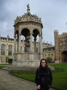
Trinity College, Cambridge.

Presenter one, Huw Price, argued that time has no arrow. It appears to in our universe: We remember the past and anticipate the future. Once a stench diffuses, it doesn’t regroup. The stench illustrates the Second Law of Thermodynamics, the assumption that entropy increases.

If “entropy” doesn’t ring a bell, never mind; we’ll dissect it in future articles. Suffice it to say that (1) thermodynamics is a branch of physics related to stat mech; (2) according to the Second Law of Thermodynamics, something called “entropy” increases; (3) entropy’s rise distinguishes the past from the future by associating the former with a low entropy and the latter with a large entropy; and (4) a stench’s diffusion illustrates the Second Law and time’s flow.

In as many universes in which entropy increases (time flows in one direction), in so many universe does entropy decrease (does time flow oppositely). So, said Huw Price, postulated the 19^th-century stat-mech founder Ludwig Boltzmann. Why would universes pair up? For the reason why, driving across a pothole, you not only fall, but also rise. Each fluctuation from equilibrium—from a flat road—involves an upward path and a downward. The upward path resembles a universe in which entropy increases; the downward, a universe in which entropy decreases. Every down pairs with an up. Averaged over universes, time has no arrow.

Freidel Weinert, presenter five, argued the opposite. Time has an arrow, he said, and not because of entropy.

Ariel Caticha discussed an impersonator of time. Using a cousin of MaxEnt, he derived an equation identical to Schrödinger’s. MaxEnt, short for “the Maximum Entropy Principle,” is a tool used in stat mech. Schrödinger’s Equation describes how quantum systems evolve. To draw from Schrödinger’s Equation predictions about electrons and atoms, physicists assume that features of reality resemble certain bits of math. We assume, for example, that the t in Schrödinger’s Equation represents time. A t appeared in Ariel’s twin of Schrödinger’s Equation. But Ariel didn’t assume what physicists usually assume. MaxEnt motivated his assumptions. Interpreting Ariel’s equation poses a challenge. If a variable acts like time and smells like time, does it represent time?**

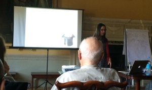
A presenter uses the anachronistic projector. The head between screen and camera belongs to David Finkelstein, who helped develop the theory of general relativity checked by Eddington.

Like Ariel, Bill Wootters questioned time’s role in arguments. The co-creator of quantum teleportation wondered why one tenet of quantum physics has the form it has. Using quantum mechanics, we can’t predict certain experiments’ outcomes. We can predict probabilities—the chance that some experiment will yield Possible Outcome 1, the chance that the experiment will yield Possible Outcome 2, and so on. To calculate these probabilities, we square numbers. Why square? Why don’t the probabilities depend on cubes?

To explore this question, Bill told a story. Suppose some experimenter runs these experiments on Monday and those on Tuesday. When evaluating his story, Bill pointed out a hole: Replacing “Monday” and “Tuesday” with “eight o’clock” and “nine” wouldn’t change his conclusion. Which replacements wouldn’t change it, and which would? To what can we generalize those days? We couldn’t answer his questions on the Sunday he asked them.

Little of presentation twelve concerned time. Rüdiger Schack introduced QBism, an interpretation of quantum mechanics that sounds like “cubism.” Casting quantum physics in terms of experimenters’ actions, Rüdiger mentioned time. By the time of the mention, I couldn’t tell what anyone meant by “time.” Raising a hand, I asked for clarification.

“You are young,” Rüdiger said. “But you will grow old and die.”

The comment clanged like the slam of a door. It echoed when I followed Ian into Ascension Parish Burial Ground. On Cambridge’s outskirts, conference-goers visited Eddington’s headstone. We found Wittgenstein’s near an uneven footpath; near tangles of undergrowth, Nobel laureates’. After debating about time, we marked its footprints. Paths of glory lead but to the grave.

Here lies one whose name was writ in a conference title: Sir Arthur Eddington’s grave.

Paths touched by little glory, I learned, have perks. As Rüdiger noted, I was the greenest participant. As he had the manners not to note, I was the least distinguished and the most ignorant. Studenthood freed me to raise my hand, to request clarification, to lack opinions about time. Perhaps I’ll evolve opinions at some t, some Monday down the road. That Monday feels infinitely far off. These days, I’ll stick to evolving science—using that other boon of youth, Facebook.

*You know you’re a theoretical physicist (or a physicist-in-training) when you debate about processes that last till kingdom come.

** As long as the variable doesn’t smell like a clogged toilet.

For videos of the presentations—including the public lecture by best-selling author Neal Stephenson—stay tuned to http://informationandinteraction.wordpress.com. My presentation appears here.

With gratitude to Ian Durham and Dean Rickles for organizing “Information and Interaction” and for the opportunity to participate. With thanks to the other participants for sharing their ideas and time.

The return of the superconducting high school teacher

Posted on May 5, 2014 by erynw

Last summer, I was blessed with the opportunity to learn about the basics of high temperature superconductors in the Yeh Group under the tutelage of visiting Professor Feng. We formed superconducting samples using a process known as Pulse Laser Deposition. We began testing the properties of the samples using X-Ray Diffraction, AC Susceptibility, and SQUIDs (superconducting quantum interference devices). I brought my new-found knowledge of these laboratory techniques and processes back into the classroom during this past school year. I was able to answer questions about the formation, research, and applications of superconductors that I had been unable to address prior to this valuable experience.

This summer I returned to the IQIM Summer Research Institute to continue my exploration of superconductors and gain even deeper research experience. This time around I have accompanied Caltech second year graduate student Kyle Chen in testing samples using the Scanning Tunneling Microscope (STM), some of which I helped form using Pulse Laser Deposition with Professor Feng last summer. I have always been curious about how we can have atomic resolution. This has been my big chance to have hands-on experience working with STM that makes it possible!

The Scanning Tunneling Microscope was invented by the late Heinrich Rohrer and Gerd Binnig at IBM Research in Zurich, Switzerland in 1981. STM is able to scan the surface contours of substances using a sharp conductive tip. The electron tunneling current through the tip of the microscope is exponentially dependent on the distance (few Angstroms) to the substance surface. The changing currents at different locations can then be compiled to produce three dimensional images of the topography of the surface on the nano-scale. Or conversely the distance can be measured while the current is held constant. STM has a much higher resolution of images and avoids the problems of diffraction and spherical aberration from lenses. This level of control and precision through STM has enabled scientists to use tools with nanometer precision, allowing scientists even to manipulate atoms and their bonds. STM has been instrumental in forming the field of nanotechnology and the modern study of DNA, semiconductors, graphene, topological insulators, and much more! Just five years after building their first STM, Rohrer and Binning’s work rightfully earned them the 1986 Nobel Prize in Physics.

Descending into the Sloan basement, Kyle and I work to prepare and scan several high temperature superconducting (HTSC) Calcium Doped YBCO $(\rm Y_{1-x} Ca_x Ba_2 Cu_3 O_{7-\delta})$ samples in order better to understand the pairing mechanism that causes Cooper Pairs for superconductivity. In regular metals, the pairing mechanism via phonon lattice vibrations is fairly well understood by physicists. Meanwhile, the pairing mechanism for HTSC is still a mystery. We are also investigating how this pairing changes with doping, as well as how the magnetic field is channeled up vortices within HTSC.

One of our first tasks is to make probe tips for STM. Adding Calcium Chloride to de-ionized water, we are preparing a liquid conductive path to begin the chemical etching of the probe tip. Using a 10V battery, a wire bent into a ring is connected to the battery and placed in the Calcium Chloride solution. Then a thin platinum iridium wire, also connected to the voltage source, is placed at the center of the conductive ring. The circuit is complete and a current of about half an Ampere is used to erode uniformly the outer surface of the platinum iridium wire, forming a sharp tip. We examine the tip under a traditional microscope to scrutinize our work. Ideally, the tip is only one atom thick! If not, we are charged with re-etching until we reach a more suitable straight, uniform, sharp tip. As we work to prepare the platinum iridium tips, a stoic picture of Neils Bohr looks down at our work with the appropriate adjacent quotation, ” When it comes to atoms, language can be used only as in poetry. The poet, too, is not nearly so concerned with describing facts as with creating images. ” After making two or three nearly perfect tips, we clean and store them in the tip case and proceed to the next step of preparation.

We are now ready to clean the sample to be tested. Bromine etching removes any oxidation or impurities that have formed on our sample, leaving a top bromine film layer. We remove the bromine-residue layer with ethanol and then plunge further into the (sub)basement to load the sample into the STM casing before oxidation begins again. The STM in the Yeh Lab was built by Professor Nai-Chang Yeh and her students eleven years ago. There are multiple layers of vacuum chambers and separate dewars, each with its own meticulous series of steps to prepare for STM testing. At the center is a long, central STM tube. Surrounding this is a large cylindrical dewar. On the perimeter is an exterior large vacuum chamber.

First we must load the newly etched YBCO sample and tip into the central STM tube. The inner tube currently lays across a work bench beneath desk lamps. We must transfer the tiny tip from the tip case to just above the sample. While loading the tip with an equally minuscule flathead screwdriver, it became quite clear to me that I could never be a surgeon! The superconducting sample is secured in place with a small cover plate and screw. A series of electronic tests for resistance and capacitance must be conducted to confirm that there are no shorts in the numerous circuits. Next we must vacuum pump the inner cylindrical tube holding the sample, tip, and circuitry until the pressure is $10^{-4}$ Bar. Then we “bake” the inner chamber, using a heater to expel any other gas, while the vacuum pump continues until we reach approximately $10^{-5}$ Bar. The heater is turned off and the vacuum continues to pump until we reach $10^{-6}$ Bar. This entire vacuum process takes approximately 15 hours…

During this span of time, I have the opportunity to observe the dark, cold STM room. The door, walls and ceiling are covered with black rubber and spongy padding to absorb vibration. The STM room is in the lowest level basement for the same reason. The vibration from human steps near the testing generates noise in the data, so every precaution is made to minimize noise. Giant cement blocks lay across the STM metal box to increase inertia and decrease noise. I ask Kyle what he usually does with this “down” time. We discuss the importance of reading equipment manuals to grasp a better understanding of the myriad of tools in the lab. He says he needs to continue reading the papers published by the Yeh Lab Group. In knowing what questions your research group has previously answered, one has a better understanding of the history and the direction of current work.

The next day, the vacuum-pumped inner chamber is loaded to the center of the STM dewar. We flush the surrounding chambers with nitrogen gas to extricate any moisture or impurities that may have entered since our last testing. Next we can set up the equipment for a liquid nitrogen transfer which lasts approximately 2 hours, depending on the transfer rate. As the liquid nitrogen is added to the system, we meticulously monitor the temperature of the STM system. It must reach 80 Kelvin before we again test the electronics. Eventually it is time to add the liquid helium. Since liquid helium is quite expensive, additional precautions are taken to ensure maximum efficiency for helium use. It is beautiful to watch the moisture in the air deposit in frost along the tubing connecting the nitrogen and helium tanks to the STM dewar. The stillness of the quiet basement as we wait for the transfer is calming. Again, we carefully monitor the temperature drop as it eventually reaches 4.2 Kelvin. For this research, STM must be cooled to this temperature because we must drop below the critical temperature of the sample in order to observe superconductivity. The lower the temperature, the more of the superconducting component manifests itself. Hence the spectrum will have higher resolution. Liquid nitrogen is first added because it can carry over 90% of the heat away due to its higher mass. Nitrogen is also significantly cheaper than liquid helium. The liquid helium is added later, because it is even cooler than liquid nitrogen.

After adding additional layers of rubber padding on top of the closed STM, we can move over to the computer that controls the STM tip. It takes approximately one hour for the tip to be slowly lowered within range for a tunneling current. Kyle examines the data from the approach to the surface. If all seems normal, we can begin the actual scan of the sample!
An important part of the lab work is trouble shooting. I have listed the ideal order of steps, but as with life, things do not always proceed as expected. I have grown in awe of the perseverance and ingenuity required for daily troubleshooting. The need to be meticulous in order to avoid error is astonishing. I love that some common household items can be a valuable tool in the lab. For example, copper scrubbers used in the kitchen serve as a simple conducting path around the inner STM chamber. Floss can be used to tie down the most delicate thin wires. I certainly have grown in my immense respect for the patience and brilliance required in real research.

I find irony in the quiet simplicity of recording and analyzing data, the stillness of carefully transferring liquid helium juxtaposed to the immense complexity and importance of this groundbreaking research. I appreciate the moments of simple quiet in the STM room, the fast paced group meetings where everyone chimes in on their progress, or the boisterous collaborative brainstorming to troubleshoot a new problem. The summer weeks in the Sloan basement have been a welcome retreat from the exciting, transformative, and exhausting year in the classroom. I am grateful for the opportunity to learn more about superconductors, quantum tunneling, vacuum pumps, sonicators, lab safety, and more. While I will not be bromine etching, chemically forming STM tips, or doing liquid helium transfers come September, I have a new-found love for the process of research that I will radiate to my students.

High School Physics Teacher Embedded on A Quest to Squash Quantum Noise

Posted on May 5, 2014 by smaloney61

Date: 8/22/2013

Location: Caltech Cryo Lab, West Bridge:

Hello: I am Steve Maloney, a Physics and Chemistry teacher intern from Duarte High School, sponsored by IQIM (Institute for Quantum Information and Matter), doing whatever I can to be of assistance to Dr. Nicolas Smith-Lefebvre. Upon meeting him in mid-June I soon learned that our mission for the length of my visit was to assist him in determining with a greater degree of certainty the linear expansion coefficient of silicon in and around 125 K. (See below)

Fig. 1: Silicon cavity.

The temperature of 125 K is of special interest to operators of LIGO (Laser Interferometer Gravitational Wave Observatory), because that is one of two temperatures where the thermal expansion coefficient, $\alpha$ , of silicon is equal to zero. A zero linear expansion coefficient is of special interest to LIGO researchers because a small change in temperature inside the cryostat, (see Fig. 2, below) will not result in a significant change in length for the silicon cavity shown in Fig. 1.

Fig. 2: Inside the Cryostat

Scientists working at LIGO need to know with great precision the length of the resonance cavity, because as gravitational waves pass through the cavity, they simultaneously compress the length of the cavity and stretch in a direction perpendicular to the shortening (warp). The arrival of a gravity wave produces a signal in the Fabry-Perot Interferometer, shown in Fig. 3, below.

Fig. 3: LIGO set-up with Fabry-Perot cavity.

Because the interferometer is sensitive to changes in length of as little as 1X10^-15m, sources of noise must be reduced to an absolute minimum. This brings us back to establishing the Thermal Coefficient of Linear Expansion, $\alpha$ . Knowing the value of $\alpha$ to a greater certainty will provide LIGO researchers the mathematical tools to better correct for small changes in temperature for the cavity, thus reducing the noise, therefore increasing the sensitivity of the Gravity Wave Detector.

So Where Do I Fit In?

In the Cryo-Lab on Thursday, July 11 2013, Nicolas Smith-Lefebvre, with my assistance, fed a radio frequency of 160.13 Mhz by means of a frequency-to-voltage transducer. The frequency fed into the transducer was changed by a fixed amount, and the change in voltage was noted. The hz / volt constant obtained was 253.9 hz / mvolt.

Nicolas then locked the east-west cryo-cavities so that the beat signal was approximately 0 (zero) volts. See the plot, below:

We then sent a 3.16 second pulse (approximated) of a 3.6 mWatt, 532 nm laser, (green) onto the surface of a mirror that reflects in the infrared, but absorbs in visible wavelengths. (Note top graph) I manufactured the electrical power interface for the laser by modifying the casing of a BIC disposable pen. The mirror was situated at the aperture of a silicon spacer.

The goal of the experiment was to determine the absorbance of the silicon mirror of the 532 nm laser.

Assuming we know the quantity of energy pulsed into the mirror:

3.6 mWatt * 3.16 s = .011376 joules,

the change in length of the cavity was determined by: Change in f/f_1550nm = change in L/ L₀

The change in volts (.025) gave us a change in f of 6.3475 x 10³ hz.

With L₀ having a value of 10 cm, that means change in L was 3.2794 x 10^-10cm.

The specific heat capacity of Si is 700j/k*kg.

Coefficient of linear expansion for Si = 2.6 x 10 ^-6/K.

To calculate increase in temperature we need to obtain the change in L.

If 2.6 x 10 ^-6/C x 10 cm x DT = DL = 3.2794 x 10^-10cm, then DT must be 1.2613 x 10 ^-5 K.

If DT = 1.2613 x 10^-5 K , then Q must equal .41 kg x 700 j/kg Kx1.2613 x 10^-5 K = 3.6 x10^-3 j,

Q/E_pulse= 3.6 x 10^-3j / 1.1376 x 10^-2j = .316 absorbance.

In other words, the silicon cavity reflected about 68% of the light that struck it.

What have I come away with from this experience?

What struck me first and foremost during this summer internship in the Cryo-Lab was the importance of future knowledge workers of having certain key skills. Among them:

Proficiency in Language

Proficiency in Math

Proficiency in Science

Proficiency in Coding

I will share my insights with my local school district and I intend to capitalize on the connections I made during my experience at Caltech.

Acknowledgements:

I would like to thank the Duarte Unified School District for giving me a leave of absence, Rana Adhikari for, yet again, finding space for me in spite of my general ineptitude regarding General Relativity, Spyridon Michalakis (Spiros) for inviting me back and letting me participate in cutting-edge science, and most of all I would like to thank Nicolas Smith-Lefebvre (softball savant), and David Yeaton-Massey (D-Mass), for their patience, generosity, and mentoring.

Hacking nature: loopholes in the laws of physics

Posted on April 29, 2014 by shaunmaguire

I spent my childhood hacking computers. When I was seven, my cousin showed up for Thanksgiving with a box filled with computer parts and we built my first computer. I got into competitive computer gaming around age eleven, and hacking was a natural extension of these activities. Then when I was sixteen, after doing poorly at a Counterstrike tournament, I decided that I should probably apply myself to other things. Needless to say, my parents were thrilled. So that’s when I bought my first computer (instead of building my own), which for deliberate but now antediluvian reasons was a Mac. A few years later, when I was taking CS 106 at Stanford, I was the first student in the course’s history whose reason for buying a Mac was “so that I couldn’t play computer games!” And now you know the story of my childhood.

The hacker mentality is quite different than the norm and my childhood trained me to look at absolutist laws as opportunities to find loopholes (of course only when legal and socially responsible!) I’ve applied this same mentality as I’ve been doing physics and I’d like to share with you some of the loopholes that I’ve gathered.

Scharnhorst effect enables light to travel faster than in vacuum (c=299,792,458 m/s): this is about the grandaddy of all laws, that nothing can travel faster than light in a vacuum! This effect is the most controversial on my list, because it hasn’t yet been experimentally verified, but it seems obvious with the right picture in mind. Most people’s mental model for light traveling in a vacuum is of little particles/waves called photons traveling through empty space. However, the vacuum is not empty! It is filled with pairs of virtual particles which momentarily fleet into existence. Interactions with these virtual particles create a small amount of ‘resistance’ as photons zoom through the vacuum (photons get absorbed into virtual electron-positron pairs and then spit back out as photons ad infinitum.) Thus, if we could somehow reduce the rate at which virtual particles are created, photons would interact less strongly with the vacuum, and would be able to travel marginally faster than c. But this is exactly what leads to the Casimir effect: the experimentally verified fact that if you take two mirrors and put them ~10 nanometers apart, then they will attract each other because there are more virtual particles created outside the cavity than inside [low momenta virtual modes are inaccessible because the uncertainty principle requires $\Delta x \cdot \Delta p= 10nm\cdot\Delta p \geq \hbar/2$ .] This effect is extremely small, only predicting that light would travel one part in $10^{36}$ faster than c. However, it should remind us all to deeply question assumptions.

This first loophole used quantum effects to beat a relativistic bound, but the next few loopholes are purely quantum, and are mainly related to that most quantum of all limits, the Heisenberg uncertainty principle.

Smashing the standard quantum limit (SQL) with squeezed measurements: the Heisenberg uncertainty principle tells us that there is a fundamental tradeoff in nature: the more precise your information about an object’s position, the less precise your knowledge about its momentum. Or vice versa, or replace x and p with E and t, or any other conjugate variables. This uncertainty principle is oftentimes written as $\Delta x\cdot \Delta p \geq \hbar/2$ . For a variety of reasons, in the early days of quantum mechanics, it was hard enough to imagine creating a state with $\Delta x \cdot \Delta p = \hbar/2$ , but there was some hope because this is obtained in the ground state of a quantum harmonic oscillator. In this case, we have $\Delta x = \Delta p = \sqrt{\hbar/2}$ . However, it was harder still to imagine creating states with $\Delta x < \sqrt{\hbar/2}$ , these states would be said to ‘go beyond the standard quantum limit’ (SQL). Over the intervening years, not only have we figured out how to go beyond the SQL using squeezed coherent states, but this is actually essential in some of our most exciting current experiments, like LIGO.

LIGO is an incredibly ambitious experiment which has been talked about multiple times on this blog. It is trying to usher in a new era of astronomy–moving beyond detecting photons–to detecting gravitational waves, ripples in spacetime which are generated as exceptionally massive objects merge, such as when two black holes collide. The effects of these waves on our local spacetime as they travel past earth are minuscule, on the scale of $10^{-18}m$ , which is about one thousand times shorter than the ‘diameter’ of a proton, and is the same order of magnitude as $\sqrt{\hbar/2}$ . Remarkably, LIGO has exploited squeezed light to demonstrate sensitivities beyond the SQL. LIGO expects to start detecting gravitational waves on a frequent basis as its upgrades deemed ‘advanced LIGO’ are completed over the next few years.

Compressed sensing beats Nyquist-Shannon: let’s play a game. Imagine I’m sending you a radio signal. How often do you need to measure the signal in order to be able to reconstruct it perfectly? The Nyquist-Shannon sampling theorem is a path-breaking result which Claude Shannon proved in 1949. If you measure at least twice as often as the highest frequency, then you are guaranteed perfect recovery of the signal. This incredibly profound result laid the foundation for modern communications. Also, it is important to realize that your signal can be much more general than simply radio waves, such as with a signal of images. This theorem is a sufficient condition for reconstruction, but is it necessary? Not even close. And it took us over 50 years to understand this in generality.

Compressed sensing was proposed between 2004-2006 by Emmanuel Candes, David Donaho and Terry Tao with important early contributions by Justin Romberg. I should note that Candes and Romberg were at Caltech during this period. The Nyquist-Shannon theorem told us that with a small amount of knowledge (a bound on the highest frequency) that we could reconstruct a signal perfectly by only measuring at a rate twice faster than the highest frequency–instead of needing to measure continuously. Compressed sensing says that with one extra assumption, assuming that only sparsely few of your frequencies are being used (call it 10 out of 1000), that you can recover your signal with high accuracy using dramatically fewer measurements. And it turns out that this assumption is valid for a huge range of applications: enabling real-time MRIs using conventional technology or more relevant to this blog, increasing our ability to distinguish quantum states via tomography.

Unlike the other topics in this blog post, I have never worked with compressed sensing, but my intuition goes like this: instead of measuring in the basis in which you are sparse (frequency for example), measure in a different basis. With high probability each of these measurements will pick up a little piece from each of the occupied modes. Then, to reconstruct your signal, you want to use the L0-“norm” to interpolate in such a way that you use the fewest frequency components possible. Computing the L0-“norm” is not efficient, so one of the major breakthroughs of compressed sensing was showing that with high probability computing the L1-norm approximates the L0 solution, and all of this can be done using a highly efficient linear program. However, I really shouldn’t be speculating because I’ve never invested much time into mastering this new tool, and I’m friends with a couple of the quantum state tomography authors, so maybe they’ll chime in?

Brahms is a cool dude. Brahms as a height map--cliffs=Gibbs phenomena=oh no! First three levels of Brahms wavelets.

Brahms is a cool dude. Brahms as a height map where cliffs=Gibbs phenomena=oh no! First three levels of Brahms as a Haar wavelet.

Wavelets as the mother of all bases: I previously wrote a post about the importance of choosing a convenient basis. Imagine you have an image which has a bunch of sharp contrasts, such as the outline of a person, or a horizon, or a table, basically anything. How do you store it efficiently? Due to the Gibbs phenomena, the Fourier basis is pretty awful for these applications. Here’s another motivating problem, imagine someone plays one note on an instrument. The sound is localized in both time and frequency. The Fourier basis is also pretty awful at storing/detecting this. Wavelets to the rescue! The theory of wavelets uses some beautiful math to solve the longstanding problem of finding a basis which is localized in both position and momenta space (or very close to it.) Wavelets have profound applications, some of my favorite include: modern image compression (JPEG 2000 onwards) is based on wavelets; Ingrid Daubechies and her colleagues used wavelets to detect forged paintings; recovering previously unrecoverable recordings of Brahms at the piano (I heard about this from Barry Simon, of Reed-Simon fame, who is currently teaching his last class ever); and even the FBI uses wavelets to compress images of fingerprints, obtaining a compression ratio of 20:1.

Postselection enables quantum cloning: the no-cloning theorem is well known in the field of quantum information. It says that you cannot find a machine (unitary operation U) which takes an arbitrary input state $|\psi\rangle$ , and a known state $|0\rangle$ , such that the machine maps $|\psi\rangle \otimes |0\rangle$ to $|\psi\rangle \otimes |\psi\rangle$ , and thereby cloning $|\psi \rangle$ . This is very easy to prove using the linearity of quantum mechanics. However, there are loopholes. One of the most trivial loopholes is realizing that one can take the state $|\psi\rangle$ and perform something called unambiguous state discrimination, which either spits out exactly which state $|\psi \rangle$ is with some probability, or otherwise spits out “I don’t know which state.” You can postselect that the unambigious state discrimination succeeded and prepare a unitary which clones the relevant states. Peter Shor has a comment on physics stackexchange describing this. Seth Lloyd and John Preskill outlined a less trivial version of this in their recent paper which tries to circumvent firewalls by using postselected quantum teleportation.

In this blog post, I’ve only described a tiny fraction of the quantum loopholes that have been discovered. If I had more space/time, two of the next examples I would describe are beating classical correlations with quantum entanglement, in order to win at CHSH games. I would also describe weak measurements and some of the peculiar things they lead to. Beyond that, I would probably refer you to Yakir Aharonov’s amazingly fun book about quantum paradoxes.

After reading this, I hope that the next time you encounter an inviolable law of nature, you’ll apply the hacker mentality and attempt to strip it down to its essence, isolate assumptions, and potentially find a loophole. But while you’re doing this, remember that you should never argue with your mother, or with mathematics!

A TED experience

Posted on April 21, 2014 by Jason Alicea

Around one year ago, I unexpectedly received an e-mail asking if I would speak at a local TEDx Youth event themed “Daring Discoveries”. I hadn’t attended a TEDx conference before (sadly I couldn’t make either of the previous ones held at Caltech). But I was familiar with the high-profile brand and so enthusiastically accepted the invitation. A few weeks ago, following a lot of preparation by the speakers and no doubt vastly more by the organizers, the event finally took place. On many levels it proved to be an unforgettable experience.

One thing that really struck me was that the conference was organized entirely by a team of local high school students. I find this truly remarkable, especially given the amount of work involved in putting together this sort of thing. (Finding speakers, fundraising, obtaining a venue, arranging innumerable technical logistics, putting together a webpage, sifting through applications, etc. I couldn’t imagine keeping track of all those details, much less at that stage!) The audience was also noteworthy: mostly other high school students from the area, their families, and other community members. In total there were about 100 participants. The vast majority reflected underrepresented groups in the sciences, which made it a particularly appealing outreach opportunity.

The organizers secured a venue at Puente Hills Mall in City of Industry. To get the mental juices flowing numerous classic brain teaser decorated the walls near the entrance. This one was my favorite:

This is an unusual paragraph. I’m curious how quickly you can find out what is so unusual about it. It looks so plain you would think nothing was wrong with it! In fact, nothing is wrong with it! It is unusual though. Study it, and think about it, but you still may not find anything odd. But if you work at it a bit, you might find out. Try to do so without any coaching.

Other interesting activities also awaited the participants, including a scavenger hunt and a “big ideas wall” where anyone could jot down ideas they viewed as worth spreading. It was fun reading what everyone had to say.

The list of speakers was eclectic and, among others, included a college student/entrepreneur, mathematicians, engineers, and educators. I found everyone’s talks absolutely riveting and felt really honored to be part of such an accomplished group. For my part I decided to tell a story about quantum computing—in particular the topological approach (what else?). Preparing was no easy task. I had to figure out a way to explain what quantum computers are, what they can do for us, why building one is hard, how “non-Abelian anyons” might one day prove to be the salvation, and why this direction is now looking increasingly promising. Of course without assuming any prior knowledge of quantum mechanics. And in about 15 minutes or so.

Given where we are in the quest for a quantum computer I had no choice but to conclude on a tentative yet optimistic note. I made sure though to convey what I think is an extremely important message. Namely, that the journey towards realizing quantum computing technology is as exciting—if not more so—than the finish line. That journey will undoubtedly be paved with groundbreaking discoveries that reveal spectacular new insights about how the universe works, forcing us to develop new physics paradigms along the way. It’s the prospect of such discoveries that energizes me to think about how we might achieve mastery over materials on large scales to hopefully overcome one of our generation’s greatest technological challenges. The Saturday Morning Breakfast Cereal comic below—which I very recently learned about from one of our colloquium speakers— perfectly encapsulates my view on the problem, both as a science advocate and a physicist working in the trenches. I thought showing this (censorship mine!) was a good message to leave the audience with.

Talking quantum mechanics with second graders

Posted on April 17, 2014 by spiros

“What’s the hardest problem you’ve ever solved?”

Kids focus right in. Driven by a ruthless curiosity, they ask questions from which adults often shy away. Which is great, if you think you know the answer to everything a 7 year-old can possibly ask you…

Two Wednesdays ago, I was invited to participate in three Q&A sessions that quickly turned into Reddit-style AMA (ask-me-anything) sessions over Skype with four 5th grade classes and one 2nd grade class of students at Medina Elementary in Medina, Washington. When asked by the organizers what I would like the sessions to focus on, I initially thought of introducing students to the mod I helped design for Minecraft, called QCraft, which brings concepts like quantum entanglement and quantum superposition into the world of Minecraft. But then I changed my mind. I told the organizers that I would talk about anything the kids wanted to know more about. It dawned on me that maybe not all 5th graders are as excited about quantum physics as I am. Yet.

The students took the bait. They peppered me with questions for over two hours —everything from “What is a quantum physicist and how do you become one?” to “What is it like to work with a fashion designer (about my collaboration with Project Runway’s Alicia Hardesty on Project X Squared)?” and of course, “Why did you steal the cannon?” (learn more about the infamous Cannon Heist – yes kids, there is an ongoing war between the two schools and Caltech took the last (hot) shot just days ago.)”

Caltech students visited MIT bearing some clever gifts.

Caltech students visited MIT during pre-frosh weekend, bearing some clever gifts.

Then they dug a little deeper: “If we have a quantum computer that knows the answer to everything, why do we need to go to school?” This question was a little tricky, so I framed the answer like this: I compared the computer to a sidekick, and the kids—the future scientists, artists and engineers —to superheroes. Sidekicks always look up to the superheroes for guidance and leadership. And then I got this question from a young girl: “If we are superheroes, what should we do with all this power?” I thought about it for a second and though my initial inclination was to go with: “You should make Angry Birds 3D!”, I went with this instead: “People often say, “Study hard so that one day you can cure cancer, figure out the theory of everything and save the world!” But I would rather see you all do things to understand the world. Sometimes you think you are saving the world when it does not need saving—it is just misunderstood. Find ways to understand one another and move to look for the value in others. Because there is always value in others, often hiding from us behind powerful emotions.” The kids listened in silence and, in that moment, I felt profoundly connected with them and their teachers.

I wasn’t expecting any more “deep” questions, until another young girl raised her hand and asked: “Can I be a quantum physicist, or is it only for the boys?” The ferocity of my answer caught me by surprise: “Of course you can! You can do anything you set your mind to and anyone who tells you otherwise, be it your teachers, your friends or even your parents, they are just wrong! In fact, you have the potential to leave all the boys in the class behind!” The applause and laughter from all the girls sounded even louder among the thunderous silence from the boys. Which is when I realized my mistake and added: “You boys can be superheroes too! Just make sure not to underestimate the girls. For your own sake.”

Why did I feel so strongly about this issue of women in science? Caltech has a notoriously bad reputation when it comes to the representation of women among our faculty and postdocs (graduate students too?) in areas such as Physics and Mathematics. IQIM has over a dozen male faculty members in its roster and only one woman: Prof. Nai-Chang Yeh. Anyone who meets Prof. Yeh quickly realizes that she is an intellectual powerhouse with boundless energy split among her research, her many students and requests for talks, conference organization and mentoring. Which is why, invariably, every one of the faculty members at IQIM feels really strongly about finding a balance and creating a more inclusive environment for women in science. This is a complex issue that requires a lot of introspection and creative ideas from all sides over the long term, but in the meantime, I just really wanted to tell the girls that I was counting on them to help with understanding our world, as much as I was counting on the boys. Quantum mechanics? They got it. Abstract math? No problem.*

It was of course inevitable that they would want to know why we created the Minecraft mod, a collaborative work between Google, MinecraftEDU and IQIM – after all, when I asked them if they had played Minecraft before, all hands shot up. Both IQIM and Google think it is important to educate younger generations about quantum computers and the complex ideas behind quantum physics; and more importantly, to meet kids where they play, in this case, inside the Minecraft game. I explained to the kids that the game was a place where they could experiment with concepts from quantum mechanics and that we were developing other resources to make sure they had a place to go to if they wanted to know more (see our animations with Jorge Cham at http://phdcomics.com/quantum).

As for the hardest problem I have ever solved? I described it in my first blog post here, An Intellectual Tornado. The kids sat listening in some sort of trance as I described the nearly perilous journey through the lands of “agony” and “self doubt” and into the valley of “grace”, the place one reaches when they learn to walk next to their worst fears, as understanding replaces fear and respect for a far superior opponent teaches true humility and instills in you a sense of adventure. By that time, I thought I was in the clear – as far as fielding difficult questions from 10 year-olds goes – but one little devil decided to ask me this simple question: “Can you explain in 2 minutes what quantum physics is?” Sure! You see kids, emptiness, what we call the quantum vacuum, underlies the emergence of spacetime through the build-up of correlations between disjoint degrees of freedom, we like to call entangled subsystems. The uniqueness of the Schmidt decomposition over generic quantum states, coupled with concentration of measure estimates over unequal bipartite decompositions gives rise to Schrodinger’s evolution and the concept of unitarity – which itself only emerges in the thermodynamic limit. In the remaining minute, let’s discuss the different interpretations of the following postulates of quantum mechanics: Let’s start with measurements…

Reaching out to elementary school kids is just one way we can make science come alive, and many of us here at IQIM look forward to sharing with kids of any age our love for adventuring far and wide to understand the world around us. In case you are an expert in anything, or just passionate about something, I highly recommend engaging the next generation through visits to classrooms and Skype sessions across state lines. Because, sometimes, you get something like this from their teacher:

Hello Dr. Michalakis,

My class was lucky enough to be able to participate in one of the Skype chats you did with Medina Elementary this morning. My students returned to the classroom with so many questions, wonderings, concerns, and ideas that we could spend the remainder of the year discussing them all.

Your ability to thoughtfully answer EVERY single question posed to you was amazing. I was so impressed and inspired by your responses that I am tempted to actually spend the remainder of the year discussing quantum mechanics J.

I particularly appreciated your point that our efforts should focus on trying to “understand the world” rather than “save” the world. I work each day to try and inspire curiosity and wonder in my students. You accomplished more towards my goal in about 40 minutes than I probably have all year. For that I am grateful.

All the best,
A.T.

* Several of my female classmates at MIT (where I did my undergraduate degree in Math with Computer Science) had a clarity of thought and a sense of perseverance that Seal Team Six would be envious of. So I would go to them for help with my hardest homework.

Tsar Nikita and His Scientists

Posted on April 14, 2014 by Nicole Yunger Halpern

Once upon a time, a Russian tsar named Nikita had forty daughters:

Every one from top to toe

Was a captivating creature,

Perfect—but for one lost feature.

So wrote Alexander Pushkin, the 19^th-century Shakespeare who revolutionized Russian literature. In a rhyme, Pushkin imagined forty princesses born without “that bit” “[b]etween their legs.” A courier scours the countryside for a witch who can help. By summoning the devil in the woods, she conjures what the princesses lack into a casket. The tsar parcels out the casket’s contents, and everyone rejoices.

“[N]onsense,” Pushkin calls the tale in its penultimate line. A “joke.”

The joke has, nearly two centuries later, become reality. Researchers have grown vaginas in a lab and implanted them into teenage girls. Thanks to a genetic defect, the girls suffered from Mayer-Rokitansky-Küster-Hauser (MRKH) syndrome: Their vaginas and uteruses had failed to grow to maturity or at all. A team at Wake Forest and in Mexico City took samples of the girls’ cells, grew more cells, and combined their harvest with vagina-shaped scaffolds. Early in the 2000s, surgeons implanted the artificial organs into the girls. The patients, the researchers reported in the journal The Lancet last week, function normally.

I don’t usually write about reproductive machinery. But the implants’ resonance with “Tsar Nikita” floored me. Scientists have implanted much of Pushkin’s plot into labs. The sexually deficient girls, the craftsperson, the replacement organs—all appear in “Tsar Nikita” as in The Lancet. In poetry as in science fiction, we read the future.

Though threads of Pushkin’s plot survive, society’s view of the specialist has progressed. “Deep [in] the dark woods” lives Pushkin’s witch. Upon summoning the devil, she locks her cure in a casket. Today’s vagina-implanters star in headlines. The Wall Street Journal highlighted the implants in its front section. Unless the patients’ health degrades, the researchers will likely list last week’s paper high on their CVs and websites.

Much as Dr. Atlántida Raya-Rivera, the paper’s lead author, differs from Pushkin’s witch, the visage of Pushkin’s magic wears the nose and eyebrows of science. When tsars or millenials need medical help, they seek knowledge-keepers: specialists, a fringe of society. Before summoning the devil, the witch “[l]ocked her door . . . Three days passed.” I hide away to calculate and study (though days alone might render me more like the protagonist in another Russian story, Chekhov’s “The Bet”). Just as the witch “stocked up coal,” some students stockpile Red Bull before hitting the library. Some habits, like the archetype of the wise woman, refuse to die.

From a Russian rhyme, the bones of “Tsar Nikita” have evolved into cutting-edge science. Pushkin and the implants highlight how attitudes toward knowledge have changed, offering a lens onto science in culture and onto science culture. No wonder readers call Pushkin “timeless.”

But what would he have rhymed with “Mayer-Rokitansky-Küster-Hauser”?

“Tsar Nikita” has many nuances—messages about censorship, for example—that I didn’t discuss. To the intrigued, I recommend The Queen of Spades: And selected works, translated by Anthony Briggs and published by Pushkin Press.

Quantum Frontiers

A blog by the Institute for Quantum Information and Matter @ Caltech

Top 10 questions for your potential PhD adviser/group

John Preskill and the dawn of the entanglement frontier

Of magnetic monopoles and fast-scrambling black holes

Clocking in at a Cambridge conference

The return of the superconducting high school teacher

High School Physics Teacher Embedded on A Quest to Squash Quantum Noise

Hacking nature: loopholes in the laws of physics

A TED experience

Talking quantum mechanics with second graders

Tsar Nikita and His Scientists

Share this:

Share this:

Share this:

Share this:

Share this:

Share this:

Share this:

Share this:

Share this:

Share this: