What is next in quantum advantage?

Posted on February 28, 2026 by Dominik Hangleiter

We are now at an exciting point in our process of developing quantum computers and understanding their computational power: It has been demonstrated that quantum computers can outperform classical ones (if you buy my argument from Parts 1 and 2 of this mini series). And it has been demonstrated that quantum fault-tolerance is possible for at least a few logical qubits. Together, these form the elementary building blocks of useful quantum computing.

And yet: the devices we have seen so far are still nowhere near being useful for any advantageous application in, say, condensed-matter physics or quantum chemistry, which is where the promise of quantum computers lies.

So what is next in quantum advantage?

This is what this third and last part of my mini-series on the question “Has quantum advantage been achieved?” is about.

The 100 logical qubits regime
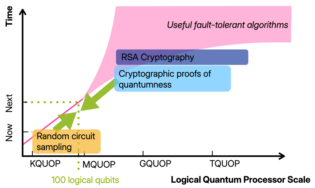
I want to have in mind the regime in which we have 100 well-functioning logical qubits, so 100 qubits on which we can run maybe 100 000 gates.

Building devices operating in this regime will require thousand(s) of physical qubits and is therefore well beyond the proof-of-principle quantum advantage and fault-tolerance experiments that have been done. At the same time, it is (so far) still one or more orders of magnitude away from any of the first applications such as simulating, say, the Fermi-Hubbard model or breaking cryptography. In other words, it is a qualitatively different regime from the early fault-tolerant computations we can do now. And yet, there is not a clear picture for what we can and should do with such devices.

The next milestone: classically verifiable quantum advantage

In this post, I want to argue that a key milestone we should aim for in the 100 logical qubit regime is classically verifiable quantum advantage. Achieving this will not only require the jump in quantum device capabilities but also finding advantage schemes that allow for classical verification using these limited resources.

Why is it an interesting and feasible goal and what is it anyway?

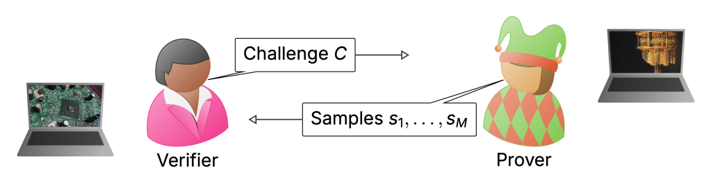
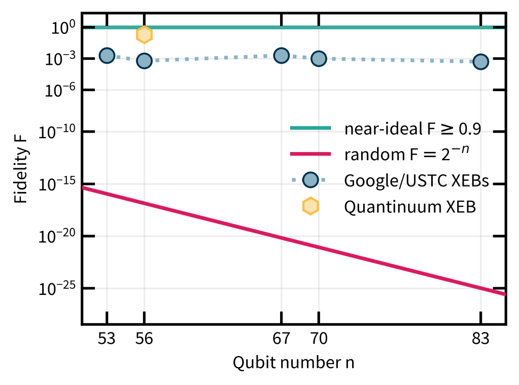
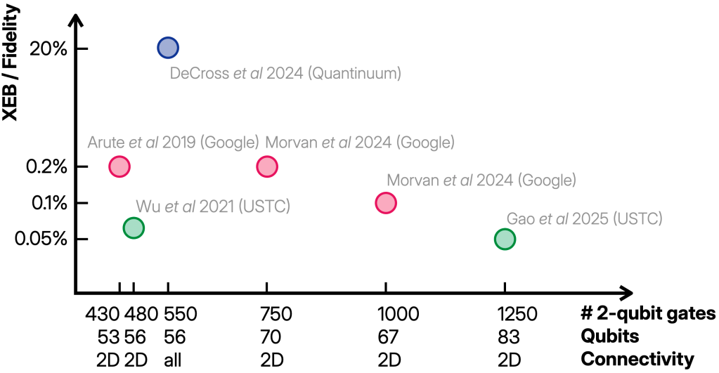
To my mind, the biggest weakness of the RCS experiments is the way they are verified. I discussed this extensively in the last posts—verification uses XEB which can be classically spoofed, and only actually measured in the simulatable regime. Really, in a quantum advantage experiment I would want there to be an efficient procedure that will without any reasonable doubt convince us that a computation must have been performed by a quantum computer when we run it. In what I think of as classically verifiable quantum advantage, a (classical) verifier would come up with challenge circuits which they would then send to a quantum server. These would be designed in such a way that once the server returns classical samples from those circuits, the verifier can convince herself that the server must have run a quantum computation.

*The theoretical computer scientist’s cartoon of verifying a quantum computer.*

This is the jump from a physics-type experiment (the sense in which advantage has been achieved) to a secure protocol that can be used in settings where I do not want to trust the server and the data it provides me with. Such security may also allow a first application of quantum computers: to generate random numbers whose genuine randomness can be certified—a task that is impossible classically.

Here is the problem: On the one hand, we do know of schemes that allow us to classically verify that a computer is quantum and generate random numbers, so called cryptographic proofs of quantumness (PoQ). A proof of quantumness is a highly reliable scheme in that its security relies on well-established cryptography. Their big drawback is that they require a large number of qubits and operations, comparable to the resources required for factoring. On the other hand, the computations we can run in the advantage regime—basically, random circuits—are very resource-efficient but not verifiable.

The 100-logical-qubit regime lies right in the middle, and it seems more than plausible that classically verifiable advantage is possible in this regime. The theory challenge ahead of us is to find it: a quantum advantage scheme that is very resource-efficient like RCS and also classically verifiable like proofs of quantumness.

*To achieve verifiable advantage in the 100-logical-qubit regime we need to close the gap between random circuit sampling and proofs of quantumness.*

With this in mind, let me spell out some concrete goals that we can achieve using 100 logical qubits on the road to classically verifiable quantum advantage.

1. Demonstrate fault-tolerant quantum advantage

Before we talk about verifiable advantage, the first experiment I would like to see is one that combines the two big achievements of the past years, and shows that quantum advantage and fault-tolerance can be achieved simultaneously. Such an experiment would be similar in type to the RCS experiments, but run on encoded qubits with gate sets that match that encoding. During the computation, noise would be suppressed by correcting for errors using the code. In doing so, we could reach the near-perfect regime of RCS as opposed to the finite-fidelity regime that current RCS experiments operate in (as I discussed in detail in Part 2).

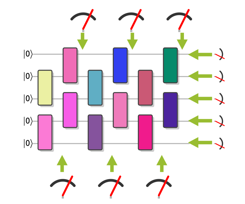
Random circuits with a quantum advantage that are particularly easy to implement fault-tolerantly are so-called IQP circuits. In those circuits, the gates are controlled-NOT gates and diagonal gates, so rotations $Z(\theta,z)$ , which just add a phase to a basis state $\ket x$ as $Z(\theta, z) \ket x = \exp(i \theta \, z \cdot x) \ket x$ . The only “quantumness” comes from the fact that each input qubit is in the superposition state $\ket + = \ket 0 + \ket 1$ , and that all qubits are measured in the $X$ basis. This is an example of an example of an IQP circuit:

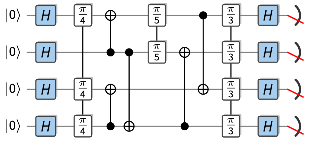
An IQP circuit starts from the all- $\ket 0$ state by applying a Hadamard transform, followed by IQP gates (in this case $Z(\pi/4,1011)$ , some CNOT gates, $Z(\pi/5,1100)$ , some CNOT gates, $Z(\pi/3,1111)$ ) and ends in a measurement in the Hadamard basis.

As it so happens, IQP circuits are already really well understood since one of the first proposals for quantum advantage was based on IQP circuits (VerIQP1), and for a lot of the results in random circuits, we have precursors for IQP circuits, in particular, their ideal and noisy complexity (SimIQP). This is because their near-classical structure makes them relatively easy to study. Most importantly, their outcome probabilities are simple (but exponentially large) sums over phases $e^{i \theta }$ that can just be read off from which gates are applied in the circuit and we can use well-established classical techniques like Boolean analysis and coding theory to understand those.

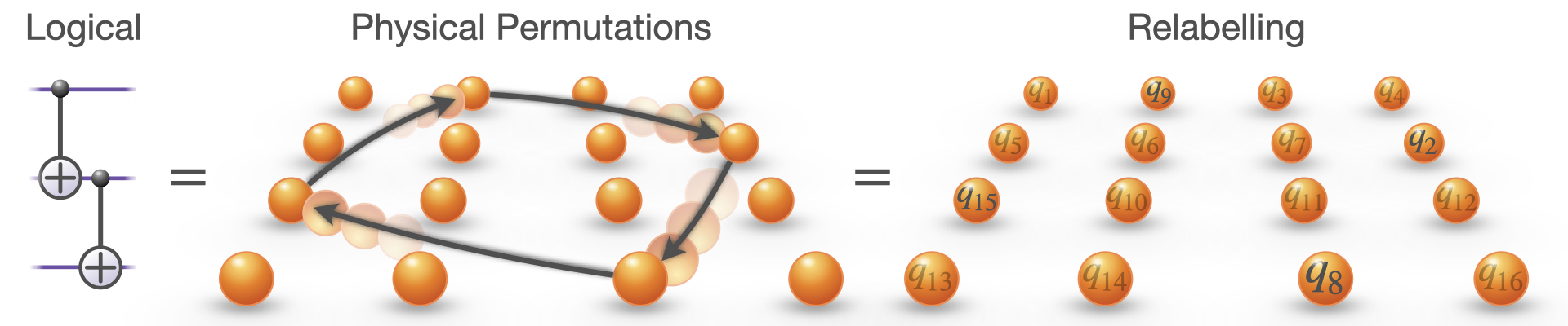
IQP gates are natural for fault-tolerance because there are codes in which all the operations involved can be implemented transversally. This means that they only require parallel physical single- or two-qubit gates to implement a logical gate rather than complicated fault-tolerant protocols which are required for universal circuits. This is in stark contrast to universal circuit which require resource-intensive fault-tolerant protocols. Running computations with IQP circuits would also be a step towards running real computations in that they can involve structured components such as cascades of CNOT gates and the like. These show up all over fault-tolerant constructions of algorithmic primitives such as arithmetic or phase estimation circuits.

Our concrete proposal for an IQP-based fault-tolerant quantum advantage experiment in reconfigurable-atom arrays is based on interleaving diagonal gates and CNOT gates to achieve super-fast scrambling (ftIQP1). A medium-size version of this protocol was implemented by the Harvard group (LogicalExp) but with only a bit more effort, it could be performed in the advantage regime.

In those proposals, verification will still suffer from the same problems of standard RCS experiments, so what’s up next is to fix that!

2. Closing the verification loophole

I said that a key milestone for the 100-logical-qubit regime is to find schemes that lie in between RCS and proofs of quantumness in terms of their resource requirements but at the same time allow for more efficient and more convincing verification than RCS. Naturally, there are two ways to approach this space—we can make quantum advantage schemes more verifiable, and we can make proofs of quantumness more resource-efficient.

First, let’s focus on the former approach and set a more moderate goal than full-on classical verification of data from an untrusted server. Are there variants of RCS that allow us to efficiently verify that finite-fidelity RCS has been achieved if we trust the experimenter and the data they hand us?

2.1 Efficient quantum verification using random circuits with symmetries

Indeed, there are! I like to think of the schemes that achieve this as random circuits with symmetries. A symmetry is an operator $S$ such that the outcome state of the computation $\ket C$ (or some intermediate state) is invariant under the symmetry, so $S \ket C =\ket C$ . The idea is then to find circuits $C$ that exhibit a quantum advantage and at the same time have symmetries that can be easily measured, say, using only single-qubit measurements or a single gate layer. Then, we can use these measurements to check whether or not the pre-measurement state respects the symmetries. This is a test for whether the quantum computer prepared the correct state, because errors or deviations from the true state would violate the symmetry (unless they were adversarially engineered).

In random circuits with symmetries, we can thus use small, well-characterized measurements whose outcomes we trust to probe whether a large quantum circuit has been run correctly. This is possible in a scenario I call the trusted experimenter scenario.

The trusted experimenter scenario
In this scenario, we receive data from an actual experiment in which we trust that certain measurements were actually and correctly performed.

*I think of random circuits with symmetries as introducing measurements in the circuit that check for errors.*

Here are some examples of random circuits with symmetries, which allow for efficient verification of quantum advantage in the trusted experimenter scenario.

Graph states. My first example are locally rotated graph states (GStates). These are states that are prepared by CZ gates acting according to the edges of a graph on an initial all- $\ket +$ state, and a layer of single-qubit $Z$ -rotations is performed before a measurement in the $X$ basis. (Yes, this is also an IQP circuit.) The symmetries of this circuit are locally rotated Pauli operators, and can therefore be measured using only single-qubit rotations and measurements. What is more, these symmetries fully determine the graph state. Determining the fidelity then just amounts to averaging the expectation values of the symmetries, which is so efficient you can even do it in your head. In this example, we need measuring the outcome state to obtain hard-to-reproduce samples and measuring the symmetries are done in two different (single-qubit) bases.

With 100 logical qubits, samples from classically intractable graph states on several 100 qubits could be easily generated.

Bell sampling. The drawback of this approach is that we need to make two different measurements for verification and sampling. But it would be much more neat if we could just verify the correctness of a set of classically hard samples by only using those samples. For an example where this is possible, consider two copies of the output state $\ket C$ of a random circuit, so $\ket C \otimes \ket C$ . This state is invariant under a swap of the two copies, and in fact the expectation value of the SWAP operator $\mathbb S$ in a noisy state preparation $\rho_C$ of $\ket C \otimes \ket C$ determines the purity of the state, so $P = \mathrm{tr}[ \rho \mathbb S]$ . It turns out that measuring all pairs of qubits in the state $\ket C \otimes \ket C$ in the pairwise basis of the four Bell states $\ket{\sigma} = (\sigma \otimes \mathbb 1) (\ket{00} + \ket{11})$ , where $\sigma$ is one of the four Pauli matrices $\mathbb 1, X, Y, Z$ , this is hard to simulate classically (BellSamp). You may also observe that the SWAP operator is diagonal in the Bell basis, so its expectation value can be extracted from the Bell-basis measurements—our hard to simulate samples. To do this, we just average sign assignments to the samples according to their parity.

If the circuit is random, then under the same assumptions as those used in XEB for random circuits, the purity is a good estimator of the fidelity, so $P \approx F(\rho_C, \ket C \otimes \ket C)$ . So here is an example, where efficient verification is possible directly from hard-to-simulate classical samples under the same assumptions as those used to argue that XEB equals fidelity.

With 100 logical qubits, we can achieve quantum advantage which is at least as hard as the current RCS experiments that can also be efficiently (physics-)verified from the classical data.

Fault-tolerant circuits. Finally, suppose that we run a fault-tolerant quantum advantage experiment. Then, there is a natural set of symmetries of the state at any point in the circuit, namely, the stabilizers of the code we use. In a fault-tolerant experiment we repeatedly measure those stabilizers mid-circuit, so why not use that data to assess the quality of the logical state? Indeed, it turns out that the logical fidelity can be estimated efficiently from stabilizer expectation values even in situations in which the logical circuit has a quantum advantage (SyndFid).

With 100 logical qubits, we could therefore just run fault-tolerant IQP circuits in the advantage regime (ftIQP1) and the syndrome data would allow us to estimate the logical fidelity.

In all of these examples of random circuits with symmetries, coming up with classical samples that pass the verification tests is very easy, so the trusted-experimenter scenario is crucial for this to work. (Note, however, that it may be possible to add tests to Bell sampling that make spoofing difficult.) At the same time, these proposals are very resource-efficient in that they only increase the cost of a pure random-circuit experiment by a relatively small amount. What is more, the required circuits have more structure than random circuits in that they typically require gates that are natural in fault-tolerant implementations of quantum algorithms.

Performing random circuit sampling with symmetries is therefore a natural next step en-route to both classically verifiable advantage that closes the no-efficient verification loophole, and towards implementing actual algorithms.

What if we do not want to afford that level of trust in the person who runs the quantum circuit, however?

2.2 Classical verification using random circuits with planted secrets

If we do not trust the experimenter, we are in the untrusted quantum server scenario.

The untrusted quantum server scenario
In this scenario, we delegate a quantum computation to an untrusted (presumably remote) quantum server—think of using a Google or Amazon cloud server to run your computation. We can communicate with this server using classical information.

In the untrusted server scenario, we can hope to use ideas from proofs of quantumness such as the use of classical cryptography to design families of quantum circuits in which some secret structure is planted. This secret structure should give the verifier a way to check whether a set of samples passes a certain verification test. At the same time it should not be detectable, or at least not be identifiable from the circuit description alone.

The simplest example of such secret structure could be a large peak in an otherwise flat output distribution of a random-looking quantum circuit. To do this, the verifier would pick a (random) string $x$ and design a circuit such that the probability of seeing $x$ in samples, is large. If the peak is hidden well, finding it just from the circuit description would require searching through all of the $2^n$ outcome bit strings and even just determining one of the outcome probabilities is exponentially difficult. A classical spoofer trying to fake the samples from a quantum computer would then be caught immediately: the list of samples they hand the verifier will not even contain $x$ unless they are unbelievably lucky, since there are exponentially many possible choices of $x$ .

Unfortunately, planting such secrets seems to be very difficult using universal circuits, since the output distributions are so unstructured. This is why we have not yet found good candidates of circuits with peaks, but some tries have been made (Peaks,ECPeaks,HPeaks)

We do have a promising candidate, though—IQP circuits! The fact that the output distributions of IQP circuits are quite simple could very well help us design sampling schemes with hidden secrets. Indeed, the idea of hiding peaks has been pioneered by Shepherd and Bremner (VerIQP1) who found a way to design classically hard IQP circuits with a large hidden Fourier coefficient. The presence of this large Fourier coefficient can easily be checked from a few classical samples, and random IQP circuits do not have any large Fourier coefficients. Unfortunately, for that construction and a variation thereof (VerIQP2), it turned out that the large coefficient can be detected quite easily from the circuit description (ClassIQP1,ClassIQP2).

To this day, it remains an exciting open question whether secrets can be planted in (maybe IQP) circuit families in a way that allows for efficient classical verification. Even finding a scheme with some large gap between verification and simulation times would be exciting, because it would for the first time allow us to verify a quantum computing experiment in the advantage regime using only classical computation.

Towards applications: certifiable random number generation

Beyond verified quantum advantage, sampling schemes with hidden secrets may be usable to generate classically certifiable random numbers: You sample from the output distribution of a random circuit with a planted secret, and verify that the samples come from the correct distribution using the secret. If the distribution has sufficiently high entropy, truly random numbers can be extracted from them. The same can be done for RCS, except that some acrobatics are needed to get around the problem that verification is just as costly as simulation (CertRand, CertRandExp). Again, a large gap between verification and simulation times would probably permit such certified random number generation.

The goal here is firstly a theoretical one: Come up with a planted-secret RCS scheme that has a large verification-simulation gap. But then, of course, it is an experimental one: actually perform such an experiment to classically verify quantum advantage.

Should an IQP-based scheme of circuits with secrets exist, 100 logical qubits is the regime where it should give a relevant advantage.

Three milestones

Altogether, I proposed three milestones for the 100 logical qubit regime.

Perform fault-tolerant quantum advantage using random IQP circuits. This will allow an improvement of the fidelity towards performing near-perfect RCS and thus closes the scalability worries of noisy quantum advantage I discussed in my last post.
Perform RCS with symmetries. This will allow for efficient verification of quantum advantage in the trusted experimenter scenario and thus make a first step toward closing the verification loophole.
Find and perform RCS schemes with planted secrets. This will allow us to verify quantum advantage in the remote untrusted server scenario and presumably give a first useful application of quantum computers to generate classically certified random numbers.

All of these experiments are natural steps towards performing actually useful quantum algorithms in that they use more structured circuits than just random universal circuits and can be used to benchmark the performance of the quantum devices in an advantage regime. Moreover, all of them close some loophole of the previous quantum advantage demonstrations, just like follow-up experiments to the first Bell tests have closed the loopholes one by one.

I argued that IQP circuits will play an important role in achieving those milestones since they are a natural circuit family in fault-tolerant constructions and promising candidates for random circuit constructions with planted secrets. Developing a better understanding of the properties of the output distributions of IQP circuits will help us achieve the theory challenges ahead.

Experimentally, the 100 logical qubit regime is exactly the regime to shoot for with those circuits since while IQP circuits are somewhat easier to simulate than universal random circuits, 100 qubits is well in the classically intractable regime.

What I did not talk about

Let me close this mini-series by touching on a few things that I would have liked to discuss more.

First, there is the OTOC experiment by the Google team (OTOC) which has spawned quite a debate. This experiment claims to achieve quantum advantage for an arguably more natural task than sampling, namely, computing expectation values. Computing expectation values is at the heart of quantum-chemistry and condensed-matter applications of quantum computers. And it has the nice property that it is what the Google team called “quantum-verifiable” (and what I would call “hopefully-in-the-future-verifiable”) in the following sense: Suppose we perform an experiment to measure a classically hard expectation value on a noisy device now, and suppose this expectation value actually carries some signal, so it is significantly far away from zero. Once we have a trustworthy quantum computer in the future, we will be able to check that the outcome of this experiment was correct and hence quantum advantage was achieved. There is a lot of interesting science to discuss about the details of this experiment and maybe I will do so in a future post.

Finally, I want to mention an interesting theory challenge that relates to the noise-scaling arguments I discussed in detail in Part 2: The challenge is to understand whether quantum advantage can be achieved in the presence of a constant amount of local noise. What do we know about this? On the one hand, log-depth random circuits with constant local noise are easy to simulate classically (SimIQP,SimRCS), and we have good numerical evidence that random circuits at very low depths are easy to simulate classically even without noise (LowDSim). So is there a depth regime in between the very low depth and the log-depth regime in which quantum advantage persists under constant local noise? Is this maybe even true in a noise regime that does not permit fault-tolerance (see this interesting talk)? In the regime in which fault-tolerance is possible, it turns out that one can construct simple fault-tolerance schemes that do not require any quantum feedback, so there are distributions that are hard to simulate classically even in the presence of constant local noise.

So long, and thanks for all the fish!

I hope that in this mini-series I could convince you that quantum advantage has been achieved. There are some open loopholes but if you are happy with physics-level experimental evidence, then you should be convinced that the RCS experiments of the past years have demonstrated quantum advantage.

As the devices are getting better at a rapid pace, there is a clear goal that I hope will be achieved in the 100-logical-qubit regime: demonstrate fault-tolerant and verifiable advantage (for the experimentalists) and come up with the schemes to do that (for the theorists)! Those experiments would close the loopholes of the current RCS experiments. And they would work as a stepping stone towards actual algorithms in the advantage regime.

I want to end with a huge thanks to Spiros Michalakis, John Preskill and Frederik Hahn who have patiently read and helped me improve these posts!

References

Fault-tolerant quantum advantage

(ftIQP1) Hangleiter, D. et al. Fault-Tolerant Compiling of Classically Hard Instantaneous Quantum Polynomial Circuits on Hypercubes. PRX Quantum 6, 020338 (2025).

(LogicalExp) Bluvstein, D. et al. Logical quantum processor based on reconfigurable atom arrays. Nature 626, 58–65 (2024).

Random circuits with symmetries

(BellSamp) Hangleiter, D. & Gullans, M. J. Bell Sampling from Quantum Circuits. Phys. Rev. Lett. 133, 020601 (2024).

(GStates) Ringbauer, M. et al. Verifiable measurement-based quantum random sampling with trapped ions. Nat Commun 16, 1–9 (2025).

(SyndFid) Xiao, X., Hangleiter, D., Bluvstein, D., Lukin, M. D. & Gullans, M. J. In-situ benchmarking of fault-tolerant quantum circuits.
I. Clifford circuits. arXiv:2601.21472
II. Circuits with a quantum advantage. (coming soon!)

Verification with planted secrets

(PoQ) Brakerski, Z., Christiano, P., Mahadev, U., Vazirani, U. & Vidick, T. A Cryptographic Test of Quantumness and Certifiable Randomness from a Single Quantum Device. in 2018 IEEE 59th Annual Symposium on Foundations of Computer Science (FOCS) 320–331 (2018).

(VerIQP1) Shepherd, D. & Bremner, M. J. Temporally unstructured quantum computation. Proceedings of the Royal Society of London A: Mathematical, Physical and Engineering Sciences 465, 1413–1439 (2009).

(VerIQP2) Bremner, M. J., Cheng, B. & Ji, Z. Instantaneous Quantum Polynomial-Time Sampling and Verifiable Quantum Advantage: Stabilizer Scheme and Classical Security. PRX Quantum 6, 020315 (2025).

(ClassIQP1) Kahanamoku-Meyer, G. D. Forging quantum data: classically defeating an IQP-based quantum test. Quantum 7, 1107 (2023).

(ClassIQP2) Gross, D. & Hangleiter, D. Secret-Extraction Attacks against Obfuscated Instantaneous Quantum Polynomial-Time Circuits. PRX Quantum 6, 020314 (2025).

(Peaks) Aaronson, S. & Zhang, Y. On verifiable quantum advantage with peaked circuit sampling. arXiv:2404.14493

(ECPeaks) Deshpande, A., Fefferman, B., Ghosh, S., Gullans, M. & Hangleiter, D. Peaked quantum advantage using error correction. arXiv:2510.05262

(HPeaks) Gharibyan, H. et al. Heuristic Quantum Advantage with Peaked Circuits. arXiv:2510.25838

Certifiable random numbers

(CertRand) Aaronson, S. & Hung, S.-H. Certified Randomness from Quantum Supremacy. in Proceedings of the 55th Annual ACM Symposium on Theory of Computing 933–944 (Association for Computing Machinery, New York, NY, USA, 2023).

(CertRandExp) Liu, M. et al. Certified randomness amplification by dynamically probing remote random quantum states. arXiv:2511.03686

OTOC

(OTOC) Abanin, D. A. et al. Observation of constructive interference at the edge of quantum ergodicity. Nature 646, 825–830 (2025).

Noisy complexity

(SimIQP) Bremner, M. J., Montanaro, A. & Shepherd, D. J. Achieving quantum supremacy with sparse and noisy commuting quantum computations. Quantum 1, 8 (2017).

(SimRCS) Aharonov, D., Gao, X., Landau, Z., Liu, Y. & Vazirani, U. A polynomial-time classical algorithm for noisy random circuit sampling. in Proceedings of the 55th Annual ACM Symposium on Theory of Computing 945–957 (2023).

(LowDSim) Napp, J. C., La Placa, R. L., Dalzell, A. M., Brandão, F. G. S. L. & Harrow, A. W. Efficient Classical Simulation of Random Shallow 2D Quantum Circuits. Phys. Rev. X 12, 021021 (2022).

Quantum cartography

Posted on February 11, 2026 by Nicole Yunger Halpern

My husband and I visited the Library of Congress on the final day of winter break this year. In a corner, we found a facsimile of a hand-drawn map: the world as viewed by sixteenth-century Europeans. North America looked like it had been dieting, having shed landmass relative to the bulk we knew. Australia didn’t appear. Yet the map’s aesthetics hit home: yellowed parchment, handwritten letters, and symbolism abounded. Never mind street view; I began hungering for an “antique” setting on Google maps.

1507 Waldseemüller Map, courtesy of the Library of Congress

Approximately four weeks after that trip, I participated in the release of another map: the publication of the review “Roadmap on quantum thermodynamics” in the journal Quantum Science and Technology. The paper contains 24 chapters, each (apart from the introduction) profiling one opportunity within the field of quantum thermodynamics. My erstwhile postdoc Aleks Lasek and I wrote the chapter about the thermodynamics of incompatible conserved quantities, as Quantum Frontiers fans¹ might guess from earlier blog posts.

Allow me to confess an ignoble truth: upon agreeing to coauthor the roadmap, I doubted whether it would impact the community enough to merit my time. Colleagues had published the book Thermodynamics in the Quantum Regime seven years earlier. Different authors had contributed different chapters, each about one topic on the rise. Did my community need such a similar review so soon after the book’s publication? If I printed a map of a city the last time I visited, should I print another map this time?

Apparently so. I often tout the swiftness with which quantum thermodynamics is developing, yet not even I predicted the appetite for the roadmap. Approximately thirty papers cited the arXiv version of the paper during the first nine months of its life—before the journal publication. I shouldn’t have likened the book and roadmap to maps of a city; I should have likened them to maps of a terra incognita undergoing exploration. Such maps change constantly, let alone over seven years.

Two trends unite many of the roadmap’s chapters, like a mountain range and a river. First, several chapters focus on experiments. Theorists founded quantum thermodynamics and dominated the field for decades, but experimentalists are turning the tables. Even theory-heavy chapters, like Aleks’s and mine, mention past experiments and experimental opportunities.

Second, several chapters blend quantum thermodynamics with many-body physics. Many-body physicists share interests with quantum thermodynamicists: thermalization and equilibrium, the absence thereof, and temperature. Yet many-body physicists belong to another tribe. They tend to interact with each other differently than quantum thermodynamicists do, write papers differently, adhere to different standards, and deploy different mathematical toolkits. Many-body-physicists use random-matrix theory, mean field theory, Wick transformations, and the like. Quantum thermodynamicists tend to cultivate and apply quantum information theory. Yet the boundary between the communities has blurred, and many scientists (including yours truly) shuttle between the two.

My favorite anti-map, from another book (series)

When Quantum Science and Technology published the roadmap, lead editor Steve Campbell announced the event to us coauthors. He’d wrangled the 69 of us into agreeing to contribute, choosing topics, drafting chapters, adhering to limitations on word counts and citations, responding to referee reports, and editing. An idiom refers to the herding of cats, but it would gain in poignancy by referring to the herding of academics. Little wonder Steve wrote in his email, “I’ll leave it to someone else to pick up the mantle and organise Roadmap #2.” I look forward to seeing that roadmap—and, perhaps, contributing to it. Who wants to pencil in Australia with me?

¹Hi, Mom and Dad.

Spooky action nearby: Entangling logical qubits without physical operations

Posted on February 2, 2026 by Shayan Majidy

**My top 10 ghosts (solo acts and ensembles).** If Bruce Willis being a ghost in *The Sixth Sense* is a spoiler, that’s on you — the movie has been out for 26 years.

Einstein and I have both been spooked by entanglement. Einstein’s experience was more profound: in a 1947 letter to Born, he famously dubbed it spukhafte Fernwirkung (or spooky action at a distance). Mine, more pedestrian. It came when I first learned the cost of entangling logical qubits on today’s hardware.

Logical entanglement is not easy

I recently listened to a talk where the speaker declared that “logical entanglement is easy,” and I have to disagree. You could argue that it looks easy when compared to logical small-angle gates, in much the same way I would look small standing next to Shaquille O’Neal. But that doesn’t mean 6’5” and 240 pounds is small.

To see why it’s not easy, it helps to look at how logical entangling gates are actually implemented. A logical qubit is not a single physical object. It’s an error-resistant qubit built out of several noisy, error-prone physical qubits. A quantum error-correcting (QEC) code with parameters $[\![n,k,d]\!]$ uses $n$ physical qubits to encode $k$ logical qubits in a way that can detect up to $d-1$ physical errors and correct up to $\lfloor (d-1)/2 \rfloor$ of them.

This redundancy is what makes fault-tolerant quantum computing possible. It’s also what makes logical operations expensive.

On platforms like neutral-atom arrays and trapped ions, the standard approach is a transversal CNOT: you apply two-qubit gates pairwise across the code blocks (qubit $i$ in block A interacts with qubit $i$ in block B). That requires $n$ physical two-qubit gates to entangle the $k$ logical qubits of one code block with the $k$ logical qubits of another.

To make this less abstract, here’s a QuEra animation showing a transversal CNOT implemented in a neutral-atom array. This animation is showing real experimental data, not a schematic idealization.

The idea is simple. The problem is that $n$ can be large, and physical two-qubit gates are among the noisiest operations available on today’s hardware.

Superconducting platforms take a different route. They tend to rely on lattice surgery; you entangle logical qubits by repeatedly measuring joint stabilizers along a boundary. That replaces two-qubit gates for stabilizer measurements over multiple rounds (typically scaling with the code distance). Unfortunately, physical measurements are the other noisiest primitive we have.

Then there are the modern high-rate qLDPC codes, which pack many logical qubits into a single code block. These are excellent quantum memories. But when it comes to computation, they face challenges. Logical entangling gates can require significant circuit depth, and often entire auxiliary code blocks are needed to mediate the interaction.

This isn’t a purely theoretical complaint. In recent state-of-the-art experiments by Google and by the Harvard–QuEra–MIT collaboration, logical entangling gates consumed nearly half of the total error budget.

So no, logical entanglement is not easy. But, how easy can we make it?

Phantom codes: Logical entanglement without physical operations

To answer how easy logical entanglement can really be, it helps to start with a slightly counterintuitive observation: logical entanglement can sometimes be generated purely by permuting physical qubits.

Let me show you how this works in the simplest possible setting, and then I’ll explain what’s really going on.

Consider a $[\![4,2,2]\!]$ stabilizer code, which encodes 4 physical qubits into 2 logical ones that can detect 1 error, but can’t correct any. Below are its logical operators; the arrow indicates what happens when we physically swap qubits 1 and 3 (bars denote logical operators).

\begin{array}{rcl} \bar X_1 &amp; = &amp; XXII \;\rightarrow\; IXXI = \bar X_1 \bar X_2 \\ \bar X_2 &amp; = &amp; XIXI \;\rightarrow\; XIXI = \bar X_2 \\ \bar Z_1 &amp; = &amp; ZIZI \;\rightarrow\; ZIZI = \bar Z_1 \\ \bar Z_2 &amp; = &amp; ZZII \;\rightarrow\; IZZI = \bar Z_1 \bar Z_2 \end{array}

You can check that the logical operators transform exactly as shown, which is the action of a logical CNOT gate. For readers less familiar with stabilizer codes, click the arrow below for an explanation of what’s going on. Those familiar can carry on.

Click!

At the logical level, we identify gates by how they transform logical Pauli operators. This is the same idea used in ordinary quantum circuits: a gate is defined not just by what it does to states, but by how it reshuffles observables.

A CNOT gate has a very characteristic action. If qubit 1 is the control and qubit 2 is the target, then: an $X$ on the control spreads to the target, a $Z$ on the target spreads back to the control, and the other Pauli operators remain unchanged.

That’s exactly what we see above.

To see why this generates entanglement, it helps to switch from operators to states. A canonical example of how to generate entanglement in quantum circuits is the following. First, you put one qubit into a superposition using a Hadamard. Starting from $|00\rangle$ , this gives

|00\rangle \rightarrow \frac{1}{\sqrt{2}}(|00\rangle + |10\rangle).

At this point there is still no entanglement — just superposition.

The entanglement appears when you apply a CNOT. The CNOT correlates the two branches of the superposition, producing

\frac{1}{\sqrt{2}}(|00\rangle + |11\rangle),

which is a maximally-entangled Bell state. The Hadamard creates superposition; the CNOT turns that superposition into correlation.

The operator transformations above are simply the algebraic version of this story. Seeing

\bar X_1 \rightarrow \bar X_1 \bar X_2 \quad {\rm and} \quad \bar Z_2 \rightarrow \bar Z_1 \bar Z_2

tells us that information on one logical qubit is now inseparable from the other.

In other words, in this code,

\bar{\rm CNOT}_{12} ={\rm SWAP}_{13}

The figure below shows how this logical circuit maps onto a physical circuit. Each horizontal line represents a qubit. On the left is a logical CNOT gate: the filled dot marks the control qubit, and the ⊕ symbol marks the target qubit whose state is flipped if the control is in the state $|1\rangle$ . On the right is the corresponding physical implementation, where the logical gate is realized by acting on multiple physical qubits.

At this point, all we’ve done is trade one physical operation for another. The real magic comes next. Physical permutations do not actually need to be implemented in hardware. Because they commute cleanly through arbitrary circuits, they can be pulled to the very end of a computation and absorbed into a relabelling of the final measurement outcomes. No operator spread. No increase in circuit depth.

This is not true for generic physical gates. It is a unique property of permutations.

To see how this works, consider a slightly larger example using an $[\![8,3,2]\!]$ code. Here the logical operators are a bit more complicated:

\bar{\rm CNOT}_{12} = {\rm SWAP}_{25}{\rm SWAP}_{37}, \quad \bar{\rm CNOT}_{23} = {\rm SWAP}_{28}{\rm SWAP}_{35}, \;\; {\rm and} \quad \;\; \bar{\rm CNOT}_{31} = {\rm SWAP}_{36}{\rm SWAP}_{45}.

Below is a three-logical-qubit circuit implemented using this code like the circuit drawn above, but now with an extra step. Suppose the circuit contains three logical CNOTs, each implemented via a physical permutation.

Instead of executing any of these permutations, we simply keep track of them classically and relabel the outputs at the end. From the hardware’s point of view, nothing happened.

If you prefer a more physical picture, imagine this implemented with atoms in an array. The atoms never move. No gates fire. The entanglement is there anyway.

This is the key point. Because no physical gates are applied, the logical entangling operation has zero overhead. And for the same reason, it has perfect fidelity. We’ve reached the minimum possible cost of a logical entangling gate. You can’t beat free.

To be clear, not all codes are amenable to logical entanglement through relabeling. This is a very special feature that exists in some codes.

Motivated by this observation, my collaborators and I defined a new class of QEC codes. I’ll state the definition first, and then unpack what it really means.

Phantom codes are stabilizer codes in which logical entangling gates between every ordered pair of logical qubits can be implemented solely via physical qubit permutations.

The phrase “every ordered pair” is a strong requirement. For three logical qubits, it means the code must support logical CNOTs between qubits $(1,2)$ , $(2,1)$ , $(1,3)$ , $(3,1)$ , $(2,3)$ , and $(3,2)$ . More generally, a code with $k$ logical qubits must support all $k(k-1)$ possible directed CNOTs. This isn’t pedantry. Without access to every directed pair, you can’t freely build arbitrary entangling circuits — you’re stuck with a restricted gate set.

The phrase “solely via physical qubit permutations” is just as demanding. If all but one of those CNOTs could be implemented via permutations, but the last one required even a single physical gate — say, a one-qubit Clifford — the code would not be phantom. That condition is what buys you zero overhead and perfect fidelity. Permutations can be compiled away entirely; any additional physical operation cannot.

Together, these two requirements carve out a very special class of codes. All in-block logical entangling gates are free. Logical entangling gates between phantom code blocks are still available — they’re simply implemented transversally.

After settling on this definition, we went back through the literature to see whether any existing codes already satisfied it. We found two. The $[\![12,2,4]\!]$ Carbon code and $[\![2^D,D,2]\!]$ hypercube codes. The former enabled repeated rounds of quantum error-correction in trapped-ion experiments, while the latter underpinned recent neutral-atom experiments achieving logical-over-physical performance gains in quantum circuit sampling.

Both are genuine phantom codes. Both are also limited. With distance $d=2$ , they can detect errors but not correct them. With only $k=2$ logical qubits, there’s a limited class of CNOT circuits you can implement. Which begs the questions: Do other phantom codes exist? Can these codes have advantages that persist for scalable applications under realistic noise conditions? What structural constraints do they obey (parameters, other gates, etc.)?

Before getting to that, a brief note for the even more expert reader on four things phantom codes are not. Phantom codes are not a form of logical Pauli-frame tracking: the phantom property survives in the presence of non-Clifford gates. They are not strictly confined to a single code block: because they are CSS codes, multiple blocks can be stitched together using physical CNOTs in linear depth. They are not automorphism gates, which rely on single-qubit Cliffords and therefore do not achieve zero overhead or perfect fidelity. And they are not codes like SHYPS, Gross, or Tesseract codes, which allow only products of CNOTs via permutations rather than individually addressable ones. All of those codes are interesting. They’re just not phantom codes.

In a recent preprint, we set out to answer the three questions above. This post isn’t about walking through all of those results in detail, so here’s the short version. First, we find many more phantom codes — hundreds of thousands of additional examples, along with infinite families that allow both $k$ and $d$ to scale. We study their structural properties and identify which other logical gates they support beyond their characteristic phantom ones.

Second, we show that phantom codes can be practically useful for the right kinds of tasks — essentially, those that are heavy on entangling gates. In end-to-end noisy simulations, we find that phantom codes can outperform the surface code, achieving one–to–two orders of magnitude reductions in logical infidelity for resource state preparation (GHZ-state preparation) and many-body simulation, at comparable qubit overhead and with a modest preselection acceptance rate of about 24%.

If you’re interested in the details, you can read more in our preprint.

Larger space of codes to explore

This is probably a good moment to zoom out and ask the referee question: why does this matter?

I was recently updating my CV and realized I’ve now written my 40th referee report for APS. After a while, refereeing trains a reflex. No matter how clever the construction or how clean the proof, you keep coming back to the same question: what does this actually change?

So why do phantom codes matter? At least to me, there are two reasons: one about how we think about QEC code design, and one about what these codes can already do in practice.

The first reason is the one I’m most excited about. It has less to do with any particular code and more to do with how the field implicitly organizes the space of QEC codes. Most of that space is structured around familiar structural properties: encoding rate, distance, stabilizer weight, LDPC-ness. These form the axes that make a code a good memory. And they matter, a lot.

But computation lives on a different axis. Logical gates cost something, and that cost is sometimes treated as downstream—something to be optimized after a code is chosen, rather than something to design for directly. As a result, the cost of logical operations is usually inherited, not engineered.

One way to make this tension explicit is to think of code design as a multi-dimensional space with at least two axes. One axis is memory cost: how efficiently a code stores information. High rate, high distance, low-weight stabilizers, efficient decoding — all the usual virtues. The other axis is computational cost: how expensive it is to actually do things with the encoded qubits. Low computational cost means many logical gates can be implemented with little overhead. Low computational cost makes computation easy.

Why focus on extreme points in this space? Because extremes are informative. They tell you what is possible, what is impossible, and which tradeoffs are structural rather than accidental.

Phantom codes sit precisely at one such extreme: they minimize the cost of in-block logical entanglement. That zero-logical-cost extreme comes with tradeoffs. The phantom codes we find tend to have high stabilizer weights, and for families with scalable $k$ , the number of physical qubits grows exponentially. These are real costs, and they matter.

Still, the important lesson is that even at this extreme point, codes can outperform LDPC-based architectures on well-chosen tasks. That observation motivates an approach to QEC code design in which the logical gates of interest are placed at the centre of the design process, rather than treated as an afterthought. This is my first takeaway from this work.

Second is that phantom codes are naturally well suited to circuits that are heavy on logical entangling gates. Some interesting applications fall into this category, including fermionic simulation and correlated-phase preparation. Combined with recent algorithmic advances that reduce the overhead of digital fermionic simulation, these code-level ideas could potentially improve near-term experimental feasibility.

Back to being spooked

The space of QEC codes is massive. Perhaps two axes are not enough. Stabilizer weight might deserve its own. Perhaps different applications demand different projections of this space. I don’t yet know the best way to organize it.

The size of this space is a little spooky — and that’s part of what makes it exciting to explore, and to see what these corners of code space can teach us about fault-tolerant quantum computation.

Has quantum advantage been achieved? Part 2: Considering the evidence

Posted on January 25, 2026 by Dominik Hangleiter

Welcome back to: Has quantum advantage been achieved?

In Part 1 of this mini-series on quantum advantage demonstrations, I told you about the idea of random circuit sampling (RCS) and the experimental implementations thereof. In this post, Part 2 out of 3, I will discuss the arguments and evidence for why I am convinced that the experiments demonstrate a quantum advantage.

Recall from Part 1 that to assess an experimental quantum advantage claim we need to check three criteria:

Does the experiment correctly solve a computational task?
Does it achieve a scalable advantage over classical computation?
Does it achieve an in-practice advantage over the best classical attempt at solving the task?

What’s the issue?

When assessing these criteria for the RCS experiments there is an important problem: The early quantum computers we ran them on were very far from being reliable and the computation was significantly corrupted by noise. How should we interpret this noisy data? Or more concisely:

Is random circuit sampling still classically hard even when we allow for whatever amount of noise the actual experiments had?
Can we be convinced from the experimental data that this task has actually been solved?

I want to convince you today that we have developed a very good understanding of these questions that gives a solid underpinning to the advantage claim. Developing that understanding required a mix of methodologies from different areas of science, including theoretical computer science, algorithm design, and physics and has been an exciting journey over the past years.

The noisy sampling task

Let us start by answering the base question. What computational task did the experiments actually solve?

Recall that, in the ideal RCS scenario, we are given a random circuit $C$ on $n$ qubits and the task is to sample from the output distribution of the state obtained $\ket C$ from applying the circuit $C$ to a simple reference state. The output probability distribution of this state is determined by the Born rule when I measure every qubit in a fixed choice of basis.

Now what does a noisy quantum computer do when I execute all the gates on it and apply them to its state? Well, it prepares a noisy version $\rho_ C$ of the intended state $\ket C$ and once I measure the qubits, I obtain samples from the output distribution of that noisy state.

We should not make the task dependent on the specifics of that state or the noise that determined it, but we can define a computational task based on this observation by fixing how accurate that noisy state preparation is. The natural way to do this is to use the fidelity

$F(C) = \bra C \rho_C \ket C,$

which is just the overlap between the ideal state and the noisy state. The fidelity is 1 if the noisy state is equal to the ideal state, and 0 if it is perfectly orthogonal to it.

Finite-fidelity random circuit sampling
Given a typical random circuit $C$ , sample from the output distribution of any quantum state whose fidelity with the ideal output state $\ket C$ is at least $\delta$ .

Note that finite-fidelity RCS does not demand success for every circuit, but only for typical circuits from the random circuit ensemble. This matches what the experiments do: they draw random circuits and need the device to perform well on the overwhelming majority of those draws. Accordingly, when the experiments quote a single number as “fidelity”, it is really the typical (or, more precisely, circuit-averaged) fidelity that I will just call $F$ .

The noisy experiments claim to have solved finite-fidelity RCS for values of $\delta$ around 0.1%. What is more, they consistently achieve this value even as the circuit sizes are increased in the later experiments. Both the actual value and the scaling will be important later.

What is the complexity of finite-fidelity RCS?

Quantum advantage of finite-fidelity RCS

Let’s start off by supposing that the quantum computation is (nearly) perfectly executed, so the required fidelity $\delta$ is quite large, say, 90%. In this scenario, we have very good evidence based on computational complexity theory that there is a scalable and in-practice quantum advantage for RCS. This evidence is very strong, comparable to the evidence we have for the hardness of factoring and simulating quantum systems. The intuition behind it is that quantum output probabilities are extremely hard to compute because of a mechanism behind quantum advantages: destructive interference. If you are interested in the subtleties and the open questions, take a look at our survey.

The question is now, how far down in fidelity this classical hardness persists? Intuitively, the smaller we make $\delta$ , the easier finite-fidelity RCS should become for a classical algorithm (and a quantum computer, too), since the freedom we have in deviating from the ideal state in our simulation becomes larger and larger. This increases the possibility of finding a state that turns out to be easy to simulate within the fidelity constraint.

Somewhat surprisingly, though, finite-fidelity RCS seems to remain hard even for very small values of $\delta$ . I am not aware of any efficient classical algorithm that achieves the finite-fidelity task for $\delta$ significantly away from the baseline trivial value of $2^{-n}$ . This is the value a maximally mixed or randomly picked state achieves because a random state has no correlation with the ideal state (or any other state), and $2^{-n}$ is exactly what you expect in that case (while 0 would correspond to perfect anti-correlation).

One can save some classical runtime compared to solving near-ideal RCS by exploiting a reduced fidelity, but the costs remain exponential. To classically solve finite-fidelity RCS, the best known approaches are reported in the papers that performed classical simulations of finite-fidelity RCS with the parameters of the first Google and USTC experiment (classSim1, classSim2). To achieve this, however, they needed to approximately simulate the ideal circuits at an immense cost. To the best of my knowledge, all but those first two experiments are far out of reach for these algorithms.

Getting the scaling right: weak noise and low depth

So what is the right value of $\delta$ at which we can hope for a scalable and in-practice advantage of RCS experiments?

When thinking about this question, it is helpful to keep a model of the circuit in mind that a noisy experiment runs. So, let us consider a noisy circuit on $n$ qubits with $d$ layers of gates and single-qubit noise of strength $\varepsilon$ on every qubit in every layer. In this scenario, the typical fidelity with the ideal state will decay as $F \sim \exp(- \varepsilon n d)$ .

Any reasonably testable value of the fidelity needs to scale as $1/\mathsf{poly}(n)$ , since eventually we need to estimate the average fidelity $F$ from the experimental samples and this typically requires at least $1/F^2$ samples, so exponentially small fidelities are experimentally invisible. The polynomial fidelity $\delta$ is also much closer to the near-ideal scenario ( $\delta \geq$ 90%) than the trivial scenario ( $\delta = 2^{-n}$ ). While we cannot formally pin this down, the intuition behind the complexity-theoretic evidence for the hardness of near-ideal RCS persists into the $\delta \sim 1/\mathsf{poly}(n)$ regime: to sample up to such high precision, we still need a reasonably accurate estimate of the ideal probabilities, and getting this is computationally extremely difficult. Scalable quantum advantage in this regime is therefore a pretty safe bet.

How do the parameters of the experiment and the RCS instances need to scale with the number of qubits $n$ to experimentally achieve the fidelity regime? The limit to consider is one in which the noise rate decreases with the number of qubits, while the circuit depth is only allowed to increase very slowly. It depends on the circuit architecture, i.e., the choice of circuit connectivity, and the gate set, through a constant $c_A$ as I will explain in more detail below.

Weak-noise and low-depth scaling
(Weak noise) The local noise rate of the quantum device scales as $\varepsilon \lt c_A/n$ .
(Low depth) The circuit depth scales as $d \lesssim \log n$ .

This limit is such that we have a scaling of the fidelity as $F \gtrsim n^{-c}$ for some constant $c$ . It is also a natural scaling limit for noisy devices whose error rates gradually improve through better engineering. You might be worried about the fact that the depth needs to be quite low but it turns out that there is a solid quantum advantage even for $\log(n)$ -depth circuits.

The precise definition of the weak-noise regime is motivated by the following observation. It turns out to be crucial for assessing the noisy data from the experiment.

Fidelity versus XEB: a phase transition

Remember from Part 1 that the experiments measured a quantity called the cross-entropy benchmark (XEB)

$\chi = 2^{2n} \mathbb E_C \mathbb E_{x} p_C(x) -1 ,$

The XEB averages the ideal probabilities $p_C(x)$ corresponding to the sampled outcomes $x$ from experiments on random circuits $C$ . Thus, it correlates the experimental and ideal output distributions of those random circuits. You can think of it as a “classical version” of the fidelity: If the experimental distribution is correct, the XEB will essentially be 1. If it is uniformly random, the XEB is 0.

The experiments claimed that the XEB is a good proxy for the circuit-averaged fidelity given by $F = \mathbb E_C F(C)$ , and so we need to understand when this is true. Fortunately, in the past few years, alongside with the improved experiments, we have developed a very good understanding of this question (WN, Spoof2, PT1, PT2).

It turns out that the quality of correspondence between XEB and average fidelity depends strongly on the noise in the experimental quantum state. In fact, there is a sharp phase transition: there is an architecture-dependent constant $c_A$ such that when the experimental local noise rate $\varepsilon < c_A/n$ , then the XEB is a good and reliable proxy for the average fidelity for any system size $n$ and circuit depth $d$ . This is exactly the weak-noise regime. Above that threshold, in the strong noise regime, the XEB is an increasingly bad proxy for the fidelity (PT1, PT2).

Let me be more precise: In the weak-noise regime, when we consider the decay of the XEB as a function of circuit depth $d$ , the rate of decay is given by $\varepsilon n$ , i.e., the XEB decays as $\exp(- \varepsilon n d )$ . Meanwhile, in the strong-noise regime the rate of decay is constant, giving an XEB decay as $\exp(- C d)$ for a constant $C$ . At the same time, the fidelity decays as $\exp(- \varepsilon n d )$ regardless of the noise regime. Hence, in the weak-noise regime, the XEB is a good proxy of the fidelity, while in the strong noise regime, there is an exponentially increasing gap between the XEB (which remains large) and the fidelity (which continues to decay exponentially). regardless of the noise regime.

This is what the following plot shows. We computed it from an exact mapping of the behavior of the XEB to the dynamics of a statistical-mechanics model that can be evaluated efficiently. Using this mapping, we can also compute the noise threshold $c_A$ for whichever random circuit family and architecture you are interested in.

From (PT2). The $y$ -axis label $\Delta( \ln \chi )$ is the decay rate of the XEB $\chi$ , $N=n$ the number of qubits and $\varepsilon$ is the local noise rate.

Where are the experiments?

We are now ready to take a look at the crux when assessing the noisy data: Can we trust the reported XEB values as an estimator of the fidelity? If so, do the experiments solve finite-fidelity RCS in the solidly hard regime where $\delta \geq 1/ \mathsf{poly}(n)$ ?

In their more recent paper (PT1), the Google team explicitly verified that the experiment is well below the phase transition, and it turns out that the first experiment was just at the boundary. The USTC experiments had comparable noise rates, and the Quantinuum experiment much better ones. Since fidelity decays as $\exp(-\varepsilon n d)$ , but the reported XEB values stayed consistently around 0.1% as $n$ was increased, the experimental error rate $\varepsilon$ of the experiments improved even better than the $1/n$ scaling required for the weak-noise regime, namely, more like $\varepsilon \sim 1/(nd)$ . Altogether, the experiments are therefore in the weak-noise regime both in terms of absolute numbers relative to $c_A/n$ and the required scaling.

Of course, to derive the transition, we made some assumptions about the noise such as that the noise is local, and that it does not depend much on the circuit itself. In the advantage experiments, these assumptions about the noise are characterized and tested. This is done through a variety of means at increasing levels of complexity, including detailed characterization of the noise in individual gates, gates run in parallel, and eventually in a larger circuit. The importance of understanding the noise shows in the fact that a significant portion of the supplementary materials of the advantage experiments is dedicated to getting this right. All of this contributes to the experimental justification for using the XEB as a proxy for the fidelity!

The data shows that the experiments solved finite-fidelity RCS for values of $\delta$ above the constant value of roughly 0.1% as the experiments grew. In the following plot, I compare the experimental fidelity values to the near-ideal scenario on the one hand, and the trivial $2^{-n}$ value on the other hand. Viewed at this scale, the values of $\delta$ for which the experiment solved finite-fidelity RCS are indeed vastly closer to the near-ideal value than the trivial baseline, which should boost our confidence that reproducing samples at a similar fidelity is extremely challenging.

The phase transition matters!

You might be tempted to say: “Well, but is all this really so important? Can’t I just use XEB and forget all about fidelity?”

The phase transition shows why that would change the complexity of the problem: in the strong-noise regime, XEB can stay high even when fidelity is exponentially small. And indeed, this discrepancy can be exploited by so-called spoofers for the XEB. These are efficient classical algorithms which can be used to succeed at a quantum advantage test even though they clearly do not achieve the intended advantage. These spoofers (Spoof1, Spoof2) can achieve high XEB scores comparable to those of the experiments and scaling like $\exp(-cd)$ in the circuit depth $d$ for some constant $c$ .

Their basic idea is to introduce strong, judiciously chosen noise at specific circuit locations that has the effect of breaking up the simulation task up into smaller, much easier components, but at the same time still gives a high XEB score. In doing so, they exploit the strong-noise regime in which the XEB is a really bad proxy for the fidelity. This allows them to sample from states with exponentially low fidelity while achieving a high XEB value.

The discovery of the phase transition and the associated spoofers highlights the importance of modeling when assessing—and even formulating—the advantage claim based on noisy data.

But we can’t compute the XEB!

You might also be worried that the experiments did not actually compute the XEB in the advantage regime because to estimate it they would have needed to compute ideal probabilities—a task that is hard by definition of the advantage regime. Instead, they used a bunch of different ways to extrapolate the true XEB from XEB proxies (proxy of a proxy of the fidelity). Is this is a valid way of getting an estimate of the true XEB?

It totally is! Different extrapolations—from easy-to-simulate to hard-to-simulate, from small system to large system etc—all gave consistent answers for the experimental XEB value of the supremacy circuits. Think of this as having several lines that cross in the same point. For that crossing to be a coincidence, something crazy, conspiratorial must happen exactly when you move to the supremacy circuits from different directions. That is why it is reasonable to trust the reported value of the XEB.

That’s exactly how experiments work!

All of this is to say that establishing that the experiments correctly solved finite-fidelity RCS and therefore show quantum advantage involved a lot of experimental characterization of the noise as well as theoretical work to understand the effects of noise on the quantity we care about—the fidelity between the experimental and ideal states.

In this respect (and maybe also in the scale of the discovery), the quantum advantage experiments are similar to the recent experiments reporting discovery of the Higgs boson and gravitational waves. While I do not claim to understand any of the details, what I do understand is that in both experiments, there is an unfathomable amount of data that could not be interpreted without preselection and post-processing of the data, theories, extrapolations and approximations that model the experiment and measurement apparatus. All of those enter the respective smoking-gun plots that show the discoveries.

If you believe in the validity of experimental physics methodology, you should therefore also believe in the type of evidence underlying experimental claim of the quantum advantage demonstrations: that they sampled from the output distribution of a quantum state with the reported fidelities.

Put succinctly: If you believe in the Higgs boson and gravitational waves, you should probably also believe in the experimental demonstration of quantum advantage.

What are the counter-arguments?

The theoretical computer scientist

“The weak-noise limit is not physical. The appropriate scaling limit is one in which the local noise rate of the device is constant while the system size grows, and in that case, there is a classical simulation algorithm for RCS (SimIQP, SimRCS).”

In theoretical computer science, scaling of time or the system size in the input size is considered very natural: We say an algorithm is efficient if its runtime and space usage only depend polynomially on the input size.

But all scaling arguments are hypothetical concepts, and we only care about the scaling at relevant sizes. In the end, every scaling limit is going to hit the wall of physical reality—be it the amount of energy or human lifetime that limits the time of an algorithm, or the physical resources that are required to build larger and larger computers. To keep the scaling limit going as we increase the size of our computations, we need innovation that makes the components smaller and less noisy.

At the scales relevant to RCS, the $1/n$ scaling of the noise is benign and even natural. Why? Well, currently, the actual noise in quantum computers is not governed by the fundamental limit, but by engineering challenges. Realizing this limit therefore amounts to engineering improvements in the system size and noise rate that are achieved over time. Sure, at some point that scaling limit is also going to hit a fundamental barrier below which the noise cannot be improved. But we are surely far away from that limit, yet. What is more, already now logical qubits are starting to work and achieve beyond-breakeven fidelities. So even if the engineering improvements should flatten out from here onward, QEC will keep the $1/n$ noise limit going and even accelerate it in the intermediate future.

The complexity maniac

“All the hard complexity-theoretic evidence for quantum advantage is in the near-ideal regime, but now you are claiming advantage for the low-fidelity version of that task.”

This is probably the strongest counter-argument in my opinion, and I gave my best response above. Let me just add that this is a question about computational complexity. In the end, all of complexity theory is based on belief. The only real evidence we have for the hardness of any task is the absence of an efficient algorithm, or the reduction to a paradigmatic, well-studied task for which there is no efficient algorithm.

I am not sure how much I would bet that you cannot find an efficient algorithm for finite-fidelity RCS in the regime of the experiments, but it is certainly a pizza.

The enthusiastic skeptic

“There is no verification test that just depends on the classical samples, is efficient and does not make any assumptions about the device. In particular, you cannot unconditionally verify fidelity just from the classical samples. Why should I believe the data?”

Yes, sure, the current advantage demonstrations are not device-independent. But the comparison you should have in mind are Bell tests. The first proper Bell tests of Aspect and others in the 80s were not free of loopholes. They still allowed for contrived explanations of the data that did not violate local realism. Still, I can hardly believe that anyone would argue that Bell inequalities were not violated already back then.

As the years passed, these remaining loopholes were closed. To be a skeptic of the data, people needed to come up with more and more adversarial scenarios that could explain the data. We are working on the same to happen with quantum advantage demonstrations: come up with better schemes and better tests that require less and less assumptions or knowledge about the specifics of the device.

The “this is unfair” argument

“When you chose the gates and architecture of the circuit dependent on your device, you tailored the task too much to the device and that is unfair. Not even the different RCS experiments solve exactly the same task.”

This is not really an argument against the achievement of quantum advantage but more against the particular choices of circuit ensembles in the experiments. Sure, the specific computations solved are still somewhat tailored to the hardware itself and in this sense the experiments are not hardware-independent yet, but they still solve fine computational tasks. Moving away from such hardware-tailored task specifications is another important next step and we are working on it.

In the third and last part of this mini series I will address next steps in quantum advantage that aim at closing some of the remaining loopholes. The most important—and theoretically interesting—one is to enable efficient verification of quantum advantage using less or even no specific knowledge about the device that was used, but just the measurement outcomes.

References

(survey) Hangleiter, D. & Eisert, J. Computational advantage of quantum random sampling. Rev. Mod. Phys. 95, 035001 (2023).

(classSim1) Pan, F., Chen, K. & Zhang, P. Solving the sampling problem of the Sycamore quantum circuits. Phys. Rev. Lett. 129, 090502 (2022).

(classSim2) Kalachev, G., Panteleev, P., Zhou, P. & Yung, M.-H. Classical Sampling of Random Quantum Circuits with Bounded Fidelity. arXiv.2112.15083 (2021).

(WN) Dalzell, A. M., Hunter-Jones, N. & Brandão, F. G. S. L. Random Quantum Circuits Transform Local Noise into Global White Noise. Commun. Math. Phys. 405, 78 (2024).

(PT1)vMorvan, A. et al. Phase transitions in random circuit sampling. Nature 634, 328–333 (2024).

(PT2) Ware, B. et al. A sharp phase transition in linear cross-entropy benchmarking. arXiv:2305.04954 (2023).

(Spoof1) Barak, B., Chou, C.-N. & Gao, X. Spoofing Linear Cross-Entropy Benchmarking in Shallow Quantum Circuits. in 12th Innovations in Theoretical Computer Science Conference (ITCS 2021) (ed. Lee, J. R.) vol. 185 30:1-30:20 (2021).

(Spoof2) Gao, X. et al. Limitations of Linear Cross-Entropy as a Measure for Quantum Advantage. PRX Quantum 5, 010334 (2024).

(SimIQP) Bremner, M. J., Montanaro, A. & Shepherd, D. J. Achieving quantum supremacy with sparse and noisy commuting quantum computations. Quantum 1, 8 (2017).

Has quantum advantage been achieved?

Posted on January 6, 2026 by Dominik Hangleiter

Recently, I gave a couple of perspective talks on quantum advantage, one at the annual retreat of the CIQC and one at a recent KITP programme. I started off by polling the audience on who believed quantum advantage had been achieved. Just this one, simple question.

The audience was mostly experimental and theoretical physicists with a few CS theory folks sprinkled in. I was sure that these audiences would be overwhelmingly convinced of the successful demonstration of quantum advantage. After all, more than half a decade has passed since the first experimental claim (G1) of “quantum supremacy” as the patron of this blog’s institute called the idea “to perform tasks with controlled quantum systems going beyond what can be achieved with ordinary digital computers” (Preskill, p. 2) back in 2012. Yes, this first experiment by the Google team may have been simulated in the meantime, but it was only the first in an impressive series of similar demonstrations that became bigger and better with every year that passed. Surely, so I thought, a significant part of my audiences would have been convinced of quantum advantage even before Google’s claim, when so-called quantum simulation experiments claimed to have performed computations that no classical computer could do (e.g. (qSim)).

I could not have been more wrong.

In both talks, less than half of the people in the audience thought that quantum advantage had been achieved.

In the discussions that ensued, I came to understand what folks criticized about the experiments that have been performed and even the concept of quantum advantage to begin with. But more on that later. Most of all, it seemed to me, the community had dismissed Google’s advantage claim because of the classical simulation shortly after. It hadn’t quite kept track of all the advances—theoretical and experimental—since then.

In a mini-series of three posts, I want to remedy this and convince you that the existing quantum computers can perform tasks that no classical computer can do. Let me caution, though, that the experiments I am going to talk about solve a (nearly) useless task. Nothing of what I say implies that you should (yet) be worried about your bank accounts.

I will start off by recapping what quantum advantage is and how it has been demonstrated in a set of experiments over the past few years.

Part 1: What is quantum advantage and what has been done?

To state the obvious: we are now fairly convinced that noiseless quantum computers would be able solve problems efficiently that no classical computer could solve. In fact, we have been convinced of that already since the mid-90ies when Lloyd and Shor discovered two basic quantum algorithms: simulating quantum systems and factoring large numbers. Both of these are tasks where we are as certain as we could be that no classical computer can solve them. So why talk about quantum advantage 20 and 30 years later?

The idea of a quantum advantage demonstration—be it on a completely useless task even—emerged as a milestone for the field in the 2010s. Achieving quantum advantage would finally demonstrate that quantum computing was not just a random idea of a bunch of academics who took quantum mechanics too seriously. It would show that quantum speedups are real: We can actually build quantum devices, control their states and the noise in them, and use them to solve tasks which not even the largest classical supercomputers could do—and these are very large.

What is quantum advantage?

But what exactly do we mean by “quantum advantage”. It is a vague concept, for sure. But some essential criteria that a demonstration should certainly satisfy are probably the following.

The quantum device needs to solve a pre-specified computational task. This means that there needs to be an input to the quantum computer. Given the input, the quantum computer must then be programmed to solve the task for the given input. This may sound trivial. But it is crucial because it delineates programmable computing devices from just experiments on any odd physical system.
There must be a scaling difference in the time it takes for a quantum computer to solve the task and the time it takes for a classical computer. As we make the problem or input size larger, the difference between the quantum and classical solution times should increase disproportionately, ideally exponentially.
And finally: the actual task solved by the quantum computer should not be solvable by any classical machine (at the time).

Achieving this last criterion using imperfect, noisy quantum devices is the challenge the idea of quantum supremacy set for the field. After all, running any of our favourite quantum algorithms in a classically hard regime on these devices is completely out of the question. They are too small and too noisy. So the field had to come up with the conceivably smallest and most noise-robust quantum algorithm that has a significant scaling advantage against classical computation.

Random circuits are really hard to simulate!

The idea is simple: we just run a random computation, constructed in a way that is as favorable as we can make it to the quantum device while being as hard as possible classically. This may strike as a pretty unfair way to come up with a computational task—it is just built to be hard for classical computers without any other purpose. But: it is a fine computational task. There is an input: the description of the quantum circuit, drawn randomly. The device needs to be programmed to run this exact circuit. And there is a task: just return whatever this quantum computation would return. These are strings of 0s and 1s drawn from a certain distribution. Getting the distribution of the strings right for a given input circuit is the computational task.

This task, dubbed random circuit sampling, can be solved on a classical as well as a quantum computer, but there is a (presumably) exponential advantage for the quantum computer. More on that in Part 2.

For now, let me tell you about the experimental demonstrations of random circuit sampling. Allow me to be slightly more formal. The task solved in random circuit sampling is to produce bit strings $x \in \{0,1\}^n$ distributed according to the Born-rule outcome distribution

$p_C(x) = | \bra x C \ket {0}|^2$

of a sequence of elementary quantum operations (unitary rotations of one or two qubits at a time) which is drawn randomly according to certain rules. This circuit $C$ is applied to a reference state $\ket 0$ on the quantum computer and then measured, giving the string $x$ as an outcome.

The breakthrough: classically hard programmable quantum computations in the real world

In the first quantum supremacy experiment (G1) by the Google team, the quantum computer was built from 53 superconducting qubits arranged in a 2D grid. The operations were randomly chosen simple one-qubit gates ( $\sqrt X, \sqrt Y, \sqrt{X+Y}$ ) and deterministic two-qubit gates called fSim applied in the 2D pattern, and repeated a certain number of times (the depth of the circuit). The limiting factor in these experiments was the quality of the two-qubit gates and the measurements, with error probabilities around 0.6 % and 4 %, respectively.

A very similar experiment was performed by the USTC team on 56 qubits (U1) and both experiments were repeated with better fidelities (0.4 % and 1 % for two-qubit gates and measurements) and slightly larger system sizes (70 and 83 qubits, respectively) in the past two years (G2,U2).

Using a trapped-ion architecture, the Quantinuum team also demonstrated random circuit sampling on 56 qubits but with arbitrary connectivity (random regular graphs) (Q). There, the two-qubit gates were $\pi/2$ -rotations around $Z \otimes Z$ , the single-qubit gates were uniformly random and the error rates much better (0.15 % for both two-qubit gate and measurement errors).

All the experiments ran random circuits on varying system sizes and circuit depths, and collected thousands to millions of samples from a few random circuits at a given size. To benchmark the quality of the samples, the widely accepted benchmark is now the linear cross-entropy (XEB) benchmark defined as

$\chi = 2^{2n} \mathbb E_C \mathbb E_{x} p_C(x) -1 ,$

for an $n$ -qubit circuit. The expectation over $C$ is over the random choice of circuit and the expectation over $x$ is over the experimental distribution of the bit strings. In other words, to compute the XEB given a list of samples, you ‘just’ need to compute the ideal probability of obtaining that sample from the circuit $C$ and average the outcomes.

The XEB is nice because it gives 1 for ideal samples from sufficiently random circuits and 0 for uniformly random samples, and it can be estimated accurately from just a few samples. Under the right conditions, it turns out to be a good proxy for the many-body fidelity of the quantum state prepared just before the measurement.

This tells us that we should expect an XEB score of $(1-\text{error per gate})^{\text{\# gates}} \sim c^{- n d }$ for some noise- and architecture-dependent constant $c$ . All of the experiments achieved a value of the XEB that was significantly (in the statistical sense) far away from 0 as you can see in the plot below. This shows that something nontrivial is going on in the experiments, because the fidelity we expect for a maximally mixed or random state is $2^{-n}$ which is less than $10^{-14}$ % for all the experiments.

The complexity of simulating these experiments is roughly governed by an exponential in either the number of qubits or the maximum bipartite entanglement generated. Figure 5 of the Quantinuum paper has a nice comparison.

It is not easy to say how much leverage an XEB significantly lower than 1 gives a classical spoofer. But one can certainly use it to judiciously change the circuit a tiny bit to make it easier to simulate.

Even then, reproducing the low scores between 0.05 % and 0.2 % of the experiments is extremely hard on classical computers. To the best of my knowledge, producing samples that match the experimental XEB score has only been achieved for the first experiment from 2019 (PCZ). This simulation already exploited the relatively low XEB score to simplify the computation, but even for the slightly larger 56 qubit experiments these techniques may not be feasibly run. So to the best of my knowledge, the only one of the experiments which may actually have been simulated is the 2019 experiment by the Google team.

If there are better methods, or computers, or more willingness to spend money on simulating random circuits today, though, I would be very excited to hear about it!

Proxy of a proxy of a benchmark

Now, you may be wondering: “How do you even compute the XEB or fidelity in a quantum advantage experiment in the first place? Doesn’t it require computing outcome probabilities of the supposedly hard quantum circuits?” And that is indeed a very good question. After all, the quantum advantage of random circuit sampling is based on the hardness of computing these probabilities. This is why, to get an estimate of the XEB in the advantage regime, the experiments needed to use proxies and extrapolation from classically tractable regimes.

This will be important for Part 2 of this series, where I will discuss the evidence we have for quantum advantage, so let me give you some more detail. To extrapolate, one can just run smaller circuits of increasing sizes and extrapolate to the size in the advantage regime. Alternatively, one can run circuits with the same number of gates but with added structure that makes them classically simulatable and extrapolate to the advantage circuits. Extrapolation is based on samples from different experiments from the quantum advantage experiments. All of the experiments did this.

A separate estimate of the XEB score is based on proxies. An XEB proxy uses the samples from the advantage experiments, but computes a different quantity than the XEB that can actually be computed and for which one can collect independent numerical and theoretical evidence that it matches the XEB in the relevant regime. For example, the Google experiments averaged outcome probabilities of modified circuits that were related to the true circuits but easier to simulate.

The Quantinuum experiment did something entirely different, which is to estimate the fidelity of the advantage experiment by inverting the circuit on the quantum computer and measuring the probability of coming back to the initial state.

All of the methods used to estimate the XEB of the quantum advantage experiments required some independent verification based on numerics on smaller sizes and induction to larger sizes, as well as theoretical arguments.

In the end, the advantage claims are thus based on a proxy of a proxy of the quantum fidelity. This is not to say that the advantage claims do not hold. In fact, I will argue in my next post that this is just the way science works. I will also tell you more about the evidence that the experiments I described here actually demonstrate quantum advantage and discuss some skeptical arguments.

Let me close this first post with a few notes.

In describing the quantum supremacy experiments, I focused on random circuit sampling which is run on programmable digital quantum computers. What I neglected to talk about is boson sampling and Gaussian boson sampling, which are run on photonic devices and have also been experimentally demonstrated. The reason for this is that I think random circuits are conceptually cleaner since they are run on processors that are in principle capable of running an arbitrary quantum computation while the photonic devices used in boson sampling are much more limited and bear more resemblance to analog simulators.

I want to continue my poll here, so feel free to write in the comments whether or not you believe that quantum advantage has been demonstrated (by these experiments) and if not, why.

References

[G1] Arute, F. et al. Quantum supremacy using a programmable superconducting processor. Nature 574, 505–510 (2019).

[Preskill] Preskill, J. Quantum computing and the entanglement frontier. arXiv:1203.5813 (2012).

[qSim] Choi, J. et al. Exploring the many-body localization transition in two dimensions. Science 352, 1547–1552 (2016). .

[U1] Wu, Y. et al. Strong Quantum Computational Advantage Using a Superconducting Quantum Processor. Phys. Rev. Lett. 127, 180501 (2021).

[G2] Morvan, A. et al. Phase transitions in random circuit sampling. Nature 634, 328–333 (2024).

[U2] Gao, D. et al. Establishing a New Benchmark in Quantum Computational Advantage with 105-qubit Zuchongzhi 3.0 Processor. Phys. Rev. Lett. 134, 090601 (2025).

[Q] DeCross, M. et al. Computational Power of Random Quantum Circuits in Arbitrary Geometries. Phys. Rev. X 15, 021052 (2025).

[PCZ] Pan, F., Chen, K. & Zhang, P. Solving the sampling problem of the Sycamore quantum circuits. Phys. Rev. Lett. 129, 090502 (2022).

Make use of time, let not advantage slip

Posted on December 14, 2025 by Nicole Yunger Halpern

During the spring of 2022, I felt as though I kept dashing backward and forward in time.

At the beginning of the season, hay fever plagued me in Maryland. Then, I left to present talks in southern California. There—closer to the equator—rose season had peaked, and wisteria petals covered the ground near Caltech’s physics building. From California, I flew to Canada to present a colloquium. Time rewound as I traveled northward; allergies struck again. After I returned to Maryland, the spring ripened almost into summer. But the calendar backtracked when I flew to Sweden: tulips and lilacs surrounded me again.

Caltech wisteria in April 2022: Thou art lovely and temperate.

The zigzagging through horticultural time disoriented my nose, but I couldn’t complain: it echoed the quantum information processing that collaborators and I would propose that summer. We showed how to improve quantum metrology—our ability to measure things, using quantum detectors—by simulating closed timelike curves.

A closed timelike curve is a trajectory that loops back on itself in spacetime. If on such a trajectory, you’ll advance forward in time, reverse chronological direction to advance backward, and then reverse again. Author Jasper Fforde illustrates closed timelike curves in his novel The Eyre Affair. A character named Colonel Next buys an edition of Shakespeare’s works, travels to the Elizabethan era, bestows them on a Brit called Will, and then returns to his family. Will copies out the plays and stages them. His colleagues publish the plays after his death, and other editions ensue. Centuries later, Colonel Next purchases one of those editions to take to the Elizabethan era.¹

Closed timelike curves can exist according to Einstein’s general theory of relativity. But do they exist? Nobody knows. Many physicists expect not. But a quantum system can simulate a closed timelike curve, undergoing a process modeled by the same mathematics.

How can one formulate closed timelike curves in quantum theory? Oxford physicist David Deutsch proposed one formulation; a team led by MIT’s Seth Lloyd proposed another. Correlations distinguish the proposals.

Two entities share correlations if a change in one entity tracks a change in the other. Two classical systems can correlate; for example, your brain is correlated with mine, now that you’ve read writing I’ve produced. Quantum systems can correlate more strongly than classical systems can, as by entangling.

Suppose Colonel Next correlates two nuclei and gives one to his daughter before embarking on his closed timelike curve. Once he completes the loop, what relationship does Colonel Next’s nucleus share with his daughter’s? The nuclei retain the correlations they shared before Colonel Next entered the loop, according to Seth and collaborators. When referring to closed timelike curves from now on, I’ll mean ones of Seth’s sort.

We can simulate closed timelike curves by subjecting a quantum system to a circuit of the type illustrated below. We read the diagram from bottom to top. Along this direction, time—as measured by a clock at rest with respect to the laboratory—progresses. Each vertical wire represents a qubit—a basic unit of quantum information, encoded in an atom or a photon or the like. Each horizontal slice of the diagram represents one instant.

At the bottom of the diagram, the two vertical wires sprout from one curved wire. This feature signifies that the experimentalist prepares the qubits in an entangled state, represented by the symbol $| \Psi_- \rangle$ . Farther up, the left-hand wire runs through a box. The box signifies that the corresponding qubit undergoes a transformation (for experts: a unitary evolution).

At the top of the diagram, the vertical wires fuse again: the experimentalist measures whether the qubits are in the state they began in. The measurement is probabilistic; we (typically) can’t predict the outcome in advance, due to the uncertainty inherent in quantum physics. If the measurement yields the yes outcome, the experimentalist has simulated a closed timelike curve. If the no outcome results, the experimentalist should scrap the trial and try again.

So much for interpreting the diagram above as a quantum circuit. We can reinterpret the illustration as a closed timelike curve. You’ve probably guessed as much, comparing the circuit diagram to the depiction, farther above, of Colonel Next’s journey. According to the second interpretation, the loop represents one particle’s trajectory through spacetime. The bottom and top show the particle reversing chronological direction—resembling me as I flew to or from southern California.

Me in southern California in spring 2022. Photo courtesy of Justin Dressel.

How can we apply closed timelike curves in quantum metrology? In Fforde’s books, Colonel Next has a brother, named Mycroft, who’s an inventor.² Suppose that Mycroft is studying how two particles interact (e.g., by an electric force). He wants to measure the interaction’s strength. Mycroft should prepare one particle—a sensor—and expose it to the second particle. He should wait for some time, then measure how much the interaction has altered the sensor’s configuration. The degree of alteration implies the interaction’s strength. The particles can be quantum, if Mycroft lives not merely in Sherlock Holmes’s world, but in a quantum-steampunk one.

But how should Mycroft prepare the sensor—in which quantum state? Certain initial states will enable the sensor to acquire ample information about the interaction; and others, no information. Mycroft can’t know which preparation will work best: the optimal preparation depends on the interaction, which he hasn’t measured yet.

Mycroft, as drawn by Sydney Paget in the 1890s

Mycroft can overcome this dilemma via a strategy published by my collaborator David Arvidsson-Shukur, his recent student Aidan McConnell, and me. According to our protocol, Mycroft entangles the sensor with a third particle. He subjects the sensor to the interaction (coupling the sensor to particle #2) and measures the sensor.

Then, Mycroft learns about the interaction—learns which state he should have prepared the sensor in earlier. He effectively teleports this state backward in time to the beginning-of-protocol sensor, using particle #3 (which began entangled with the sensor).³ Quantum teleportation is a decades-old information-processing task that relies on entanglement manipulation. The protocol can transmit quantum states over arbitrary distances—or, effectively, across time.

We can view Mycroft’s experiment in two ways. Using several particles, he manipulates entanglement to measure the interaction strength optimally (with the best possible precision). This process is mathematically equivalent to another. In the latter process, Mycroft uses only one sensor. It comes forward in time, reverses chronological direction (after Mycroft learns the optimal initial state’s form), backtracks to an earlier time (to when the sensing protocol began), and returns to progressing forward in time (informing Mycroft about the interaction).

Where I stayed in Stockholm. I swear, I’m not making this up.

In Sweden, I regarded my work with David and Aidan as a lark. But it’s led to an experiment, another experiment, and two papers set to debut this winter. I even pass as a quantum metrologist nowadays. Perhaps I should have anticipated the metamorphosis, as I should have anticipated the extra springtimes that erupted as I traveled between north and south. As the bard says, there’s a time for all things.

¹In the sequel, Fforde adds a twist to Next’s closed timelike curve. I can’t speak for the twist’s plausibility or logic, but it makes for delightful reading, so I commend the novel to you.

²You might recall that Sherlock Holmes has a brother, named Mycroft, who’s an inventor. Why? In Fforde’s novel, an evil corporation pursues Mycroft, who’s built a device that can transport him into the world of a book. Mycroft uses the device to hide from the corporation in Sherlock Holmes’s backstory.

³Experts, Mycroft implements the effective teleportation as follows: He prepares a fourth particle in the ideal initial sensor state. Then, he performs a two-outcome entangling measurement on particles 3 and 4: he asks “Are particles 3 and 4 in the state in which particles 1 and 3 began?” If the measurement yields the yes outcome, Mycroft has effectively teleported the ideal sensor state backward in time. He’s also simulated a closed timelike curve. If the measurement yields the no outcome, Mycroft fails to measure the interaction optimally. Figure 1 in our paper synopsizes the protocol.

What distinguishes quantum from classical thermodynamics?

Posted on November 26, 2025 by Nicole Yunger Halpern

Should you require a model for an Oxford don in a play or novel, look no farther than Andrew Briggs. The emeritus professor of nanomaterials speaks with a southern-English accent as crisp as shortbread, exhibits manners to which etiquette influencer William Hanson could aspire, and can discourse about anything from Bantu to biblical Hebrew. I joined Andrew for lunch at St. Anne’s College, Oxford, this month.¹ Over vegetable frittata, he asked me what unifying principle distinguishes quantum from classical thermodynamics.

With a thermodynamic colleague at the Oxford University Museum of Natural History

I’d approached quantum thermodynamics from nearly every angle I could think of. I’d marched through the thickets of derivations and plots; I’d journeyed from subfield to subfield; I’d gazed down upon the discipline as upon a landscape from a hot-air balloon. I’d even prepared a list of thermodynamic tasks enhanced by quantum phenomena: we can charge certain batteries at greater powers if we entangle them than if we don’t, entanglement can raise the amount of heat pumped out of a system by a refrigerator, etc. But Andrew’s question flummoxed me.

I bungled the answer. I toted out the aforementioned list, but it contained examples, not a unifying principle. The next day, I was sitting in an office borrowed from experimentalist Natalia Ares in New College, a Gothic confection founded during the late 1300s (as one should expect of a British college called “New”). Admiring the view of ancient stone walls, I realized how I should have responded the previous day.

View from a window near the office I borrowed in New College. If I could pack that office in a suitcase and carry it home, I would.

My answer begins with a blog post written in response to a quantum-thermodynamics question from a don at another venerable university: Yoram Alhassid. He asked, “What distinguishes quantum thermodynamics to quantum statistical mechanics?” You can read the full response here. Takeaways include thermodynamics’s operational flavor. When using an operational theory, we imagine agents who perform tasks, using given resources. For example, a thermodynamic agent may power a steamboat, given a hot gas and a cold gas. We calculate how effectively the agents can perform those tasks. For example, we compute heat engines’ efficiencies. If a thermodynamic agent can access quantum resources, I’ll call them “quantum thermodynamic.” If the agent can access only everyday resources, I’ll call them “classical thermodynamic.”

A quantum thermodynamic agent may access more resources than a classical thermodynamic agent can. The latter can leverage work (well-organized energy), free energy (the capacity to perform work), information, and more. A quantum agent may access not only those resources, but also entanglement (strong correlations between quantum particles), coherence (wavelike properties of quantum systems), squeezing (the ability to toy with quantum uncertainty as quantified by Heisenberg and others), and more. The quantum-thermodynamic agent may apply these resources as described in the list I rattled off at Andrew.

With Oxford experimentalist Natalia Ares in her lab

Yet quantum phenomena can impede a quantum agent in certain scenarios, despite assisting the agent in others. For example, coherence can reduce a quantum engine’s power. So can noncommutation. Everyday numbers commute under multiplication: 11 times 12 equals 12 times 11. Yet quantum physics features numbers that don’t commute so. This noncommutation underlies quantum uncertainty, quantum error correction, and much quantum thermodynamics blogged about ad nauseam on Quantum Frontiers. A quantum engine’s dynamics may involve noncommutation (technically, the Hamiltonian may contain terms that fail to commute with each other). This noncommutation—a fairly quantum phenomenon—can impede the engine similarly to friction. Furthermore, some quantum thermodynamic agents must fight decoherence, the leaking of quantum information from a quantum system into its environment. Decoherence needn’t worry any classical thermodynamic agent.

In short, quantum thermodynamic agents can benefit from more resources than classical thermodynamic agents can, but the quantum agents also face more threats. This principle might not encapsulate how all of quantum thermodynamics differs from its classical counterpart, but I think the principle summarizes much of the distinction. And at least I can posit such a principle. I didn’t have enough experience when I first authored a blog post about Oxford, in 2013. People say that Oxford never changes, but this quantum thermodynamic agent does.

In the University of Oxford Natural History Museum in 2013, 2017, and 2025. I’ve published nearly 150 Quantum Frontiers posts since taking the first photo!

¹Oxford consists of colleges similarly to how neighborhoods form a suburb. Residents of multiple neighborhoods may work in the same dental office. Analogously, faculty from multiple colleges may work, and undergraduates from multiple colleges may major, in the same department.

A (quantum) complex legacy: Part trois

Posted on June 22, 2025 by Nicole Yunger Halpern

When I worked in Cambridge, Massachusetts, a friend reported that MIT’s postdoc association had asked its members how it could improve their lives. The friend confided his suggestion to me: throw more parties.¹ This year grants his wish on a scale grander than any postdoc association could. The United Nations has designated 2025 as the International Year of Quantum Science and Technology (IYQ), as you’ve heard unless you live under a rock (or without media access—which, come to think of it, sounds not unappealing).

A metaphorical party cracker has been cracking since January. Governments, companies, and universities are trumpeting investments in quantum efforts. Institutions pulled out all the stops for World Quantum Day, which happens every April 14 but which scored a Google doodle this year. The American Physical Society (APS) suffused its Global Physics Summit in March with quantum science like a Bath & Body Works shop with the scent of Pink Pineapple Sunrise. At the summit, special symposia showcased quantum research, fellow blogger John Preskill dished about quantum-science history in a dinnertime speech, and a “quantum block party” took place one evening. I still couldn’t tell you what a quantum block party is, but this one involved glow sticks.

Attending the summit, I felt a satisfaction—an exultation, even—redolent of twelfth grade, when American teenagers summit the Mont Blanc of high school. It was the feeling that this year is our year. Pardon me while I hum “Time of your life.”²

Speakers and organizer of a Kavli Symposium, a special session dedicated to interdisciplinary quantum science, at the APS Global Physics Summit

Just before the summit, editors of the journal PRX Quantum released a special collection in honor of the IYQ.³ The collection showcases a range of advances, from chemistry to quantum error correction and from atoms to attosecond-length laser pulses. Collaborators and I contributed a paper about quantum complexity, a term that has as many meanings as companies have broadcast quantum news items within the past six months. But I’ve already published two Quantum Frontiers posts about complexity, and you surely study this blog as though it were the Bible, so we’re on the same page, right?

Just joshing.

Imagine you have a quantum computer that’s running a circuit. The computer consists of qubits, such as atoms or ions. They begin in a simple, “fresh” state, like a blank notebook. Post-circuit, they store quantum information, such as entanglement, as a notebook stores information post-semester. We say that the qubits are in some quantum state. The state’s quantum complexity is the least number of basic operations, such as quantum logic gates, needed to create that state—via the just-completed circuit or any other circuit.

Today’s quantum computers can’t create high-complexity states. The reason is, every quantum computer inhabits an environment that disturbs the qubits. Air molecules can bounce off them, for instance. Such disturbances corrupt the information stored in the qubits. Wait too long, and the environment will degrade too much of the information for the quantum computer to work. We call the threshold time the qubits’ lifetime, among more-obscure-sounding phrases. The lifetime limits the number of gates we can run per quantum circuit.

The ability to perform many quantum gates—to perform high-complexity operations—serves as a resource. Other quantities serve as resources, too, as you’ll know if you’re one of the three diehard Quantum Frontiers fans who’ve been reading this blog since 2014 (hi, Mom). Thermodynamic resources include work: coordinated energy that one can harness directly to perform a useful task, such as lifting a notebook or staying up late enough to find out what a quantum block party is.

My collaborators: Jonas Haferkamp, Philippe Faist, Teja Kothakonda, Jens Eisert, and Anthony Munson (in an order of no significance here)

My collaborators and I showed that work trades off with complexity in information- and energy-processing tasks: the more quantum gates you can perform, the less work you have to spend on a task, and vice versa. Qubit reset exemplifies such tasks. Suppose you’ve filled a notebook with a calculation, you want to begin another calculation, and you have no more paper. You have to erase your notebook. Similarly, suppose you’ve completed a quantum computation and you want to run another quantum circuit. You have to reset your qubits to a fresh, simple state.

Three methods suggest themselves. First, you can “uncompute,” reversing every quantum gate you performed.⁴ This strategy requires a long lifetime: the information imprinted on the qubits by a gate mustn’t leak into the environment before you’ve undone the gate.

Second, you can do the quantum equivalent of wielding a Pink Pearl Paper Mate: you can rub the information out of your qubits, regardless of the circuit you just performed. Thermodynamicists inventively call this strategy erasure. It requires thermodynamic work, just as applying a Paper Mate to a notebook does.

Third, you can

Suppose your qubits have finite lifetimes. You can undo as many gates as you have time to. Then, you can erase the rest of the qubits, spending work. How does complexity—your ability to perform many gates—trade off with work? My collaborators and I quantified the tradeoff in terms of an entropy we invented because the world didn’t have enough types of entropy.⁵

Complexity trades off with work not only in qubit reset, but also in data compression and likely other tasks. Quantum complexity, my collaborators and I showed, deserves a seat at the great soda fountain of quantum thermodynamics.

The great soda fountain of quantum thermodynamics

…as quantum information science deserves a seat at the great soda fountain of physics. When I embarked upon my PhD, faculty members advised me to undertake not only quantum-information research, but also some “real physics,” such as condensed matter. The latter would help convince physics departments that I was worth their money when I applied for faculty positions. By today, the tables have turned. A condensed-matter theorist I know has wound up an electrical-engineering professor because he calculates entanglement entropies.

So enjoy our year, fellow quantum scientists. Party like it’s 1925. Burnish those qubits—I hope they achieve the lifetimes of your life.

¹Ten points if you can guess who the friend is.

²Whose official title, I didn’t realize until now, is “Good riddance.” My conception of graduation rituals has just turned a somersault.

³PR stands for Physical Review, the brand of the journals published by the APS. The APS may have intended for the X to evoke exceptional, but I like to think it stands for something more exotic-sounding, like ex vita discedo, tanquam ex hospitio, non tanquam ex domo.

⁴Don’t ask me about the notebook analogue of uncomputing a quantum state. Explaining it would require another blog post.

⁵For more entropies inspired by quantum complexity, see this preprint. You might recognize two of the authors from earlier Quantum Frontiers posts if you’re one of the three…no, not even the three diehard Quantum Frontiers readers will recall; but trust me, two of the authors have received nods on this blog before.

The most steampunk qubit

Posted on May 25, 2025 by Nicole Yunger Halpern

I never imagined that an artist would update me about quantum-computing research.

Last year, steampunk artist Bruce Rosenbaum forwarded me a notification about a news article published in Science. The article reported on an experiment performed in physicist Yiwen Chu’s lab at ETH Zürich. The experimentalists had built a “mechanical qubit”: they’d stored a basic unit of quantum information in a mechanical device that vibrates like a drumhead. The article dubbed the device a “steampunk qubit.”

I was collaborating with Bruce on a quantum-steampunk sculpture, and he asked if we should incorporate the qubit into the design. Leave it for a later project, I advised. But why on God’s green Earth are you receiving email updates about quantum computing?

My news feed sends me everything that says “steampunk,” he explained. So keeping a bead on steampunk can keep one up to date on quantum science and technology—as I’ve been preaching for years.

Other ideas displaced Chu’s qubit in my mind until I visited the University of California, Berkeley this January. Visiting Berkeley in January, one can’t help noticing—perhaps with a trace of smugness—the discrepancy between the temperature there and the temperature at home. And how better to celebrate a temperature difference than by studying a quantum-thermodynamics-style throwback to the 1800s?

One sun-drenched afternoon, I learned that one of my hosts had designed another steampunk qubit: Alp Sipahigil, an assistant professor of electrical engineering. He’d worked at Caltech as a postdoc around the time I’d finished my PhD there. We’d scarcely interacted, but I’d begun learning about his experiments in atomic, molecular, and optical physics then. Alp had learned about my work through Quantum Frontiers, as I discovered this January. I had no idea that he’d “met” me through the blog until he revealed as much to Berkeley’s physics department, when introducing the colloquium I was about to present.

Alp and collaborators proposed that a qubit could work as follows. It consists largely of a cantilever, which resembles a pendulum that bobs back and forth. The cantilever, being quantum, can have only certain amounts of energy. When the pendulum has a particular amount of energy, we say that the pendulum is in a particular energy level.

One might hope to use two of the energy levels as a qubit: if the pendulum were in its lowest-energy level, the qubit would be in its 0 state; and the next-highest level would represent the 1 state. A bit—a basic unit of classical information—has 0 and 1 states. A qubit can be in a superposition of 0 and 1 states, and so the cantilever could be.

A flaw undermines this plan, though. Suppose we want to process the information stored in the cantilever—for example, to turn a 0 state into a 1 state. We’d inject quanta—little packets—of energy into the cantilever. Each quantum would contain an amount of energy equal to (the energy associated with the cantilever’s 1 state) – (the amount associated with the 0 state). This equality would ensure that the cantilever could accept the energy packets lobbed at it.

But the cantilever doesn’t have only two energy levels; it has loads. Worse, all the inter-level energy gaps equal each other. However much energy the cantilever consumes when hopping from level 0 to level 1, it consumes that much when hopping from level 1 to level 2. This pattern continues throughout the rest of the levels. So imagine starting the cantilever in its 0 level, then trying to boost the cantilever into its 1 level. We’d probably succeed; the cantilever would probably consume a quantum of energy. But nothing would stop the cantilever from gulping more quanta and rising to higher energy levels. The cantilever would cease to serve as a qubit.

We can avoid this problem, Alp’s team proposed, by placing an atomic-force microscope near the cantilever. An atomic force microscope maps out surfaces similarly to how a Braille user reads: by reaching out a hand and feeling. The microscope’s “hand” is a tip about ten nanometers across. So the microscope can feel surfaces far more fine-grained than a Braille user can. Bumps embossed on a page force a Braille user’s finger up and down. Similarly, the microscope’s tip bobs up and down due to forces exerted by the object being scanned.

Imagine placing a microscope tip such that the cantilever swings toward it and then away. The cantilever and tip will exert forces on each other, especially when the cantilever swings close. This force changes the cantilever’s energy levels. Alp’s team chose the tip’s location, the cantilever’s length, and other parameters carefully. Under the chosen conditions, boosting the cantilever from energy level 1 to level 2 costs more energy than boosting from 0 to 1.

So imagine, again, preparing the cantilever in its 0 state and injecting energy quanta. The cantilever will gobble a quantum, rising to level 1. The cantilever will then remain there, as desired: to rise to level 2, the cantilever would have to gobble a larger energy quantum, which we haven’t provided.¹

Will Alp build the mechanical qubit proposed by him and his collaborators? Yes, he confided, if he acquires a student nutty enough to try the experiment. For when he does—after the student has struggled through the project like a dirigible through a hurricane, but ultimately triumphed, and a journal is preparing to publish their magnum opus, and they’re brainstorming about artwork to represent their experiment on the journal’s cover—I know just the aesthetic to do the project justice.

¹Chu’s team altered their cantilever’s energy levels using a superconducting qubit, rather than an atomic force microscope.

Quantum automata

Posted on April 27, 2025 by Nicole Yunger Halpern

Do you know when an engineer built the first artificial automaton—the first human-made machine that operated by itself, without external control mechanisms that altered the machine’s behavior over time as the machine undertook its mission?

The ancient Greek thinker Archytas of Tarentum reportedly created it about 2,300 years ago. Steam propelled his mechanical pigeon through the air.

For centuries, automata cropped up here and there as curiosities and entertainment. The wealthy exhibited automata to amuse and awe their peers and underlings. For instance, the French engineer Jacques de Vauconson built a mechanical duck that appeared to eat and then expel grains. The device earned the nickname the Digesting Duck…and the nickname the Defecating Duck.

Vauconson also invented a mechanical loom that helped foster the Industrial Revolution. During the 18th and 19th centuries, automata began to enable factories, which changed the face of civilization. We’ve inherited the upshots of that change. Nowadays, cars drive themselves, Roombas clean floors, and drones deliver packages.¹ Automata have graduated from toys to practical tools.²

Rather, classical automata have. What of their quantum counterparts?

Scientists have designed autonomous quantum machines, and experimentalists have begun realizing them. The roster of such machines includes autonomous quantum engines, refrigerators, and clocks. Much of this research falls under the purview of quantum thermodynamics, due to the roles played by energy in these machines’ functioning: above, I defined an automaton as a machine free of time-dependent control (exerted by a user). Equivalently, according to a thermodynamicist mentality, we can define an automaton as a machine on which no user performs any work as the machine operates. Thermodynamic work is well-ordered energy that can be harnessed directly to perform a useful task. Often, instead of receiving work, an automaton receives access to a hot environment and a cold environment. Heat flows from the hot to the cold, and the automaton transforms some of the heat into work.

Quantum automata appeal to me because quantum thermodynamics has few practical applications, as I complained in my previous blog post. Quantum thermodynamics has helped illuminate the nature of the universe, and I laud such foundational insights. Yet we can progress beyond laudation by trying to harness those insights in applications. Some quantum thermal machines—quantum batteries, engines, etc.—can outperform their classical counterparts, according to certain metrics. But controlling those machines, and keeping them cold enough that they behave quantum mechanically, costs substantial resources. The machines cost more than they’re worth. Quantum automata, requiring little control, offer hope for practicality.

To illustrate this hope, my group partnered with Simone Gasparinetti’s lab at Chalmer’s University in Sweden. The experimentalists created an autonomous quantum refrigerator from superconducting qubits. The quantum refrigerator can help reset, or “clear,” a quantum computer between calculations.

Artist’s conception of the autonomous-quantum-refrigerator chip. Credit: Chalmers University of Technology/Boid AB/NIST.

After we wrote the refrigerator paper, collaborators and I raised our heads and peered a little farther into the distance. What does building a useful autonomous quantum machine take, generally? Collaborators and I laid out guidelines in a “Key Issues Review” published in Reports in Progress on Physics last November.

We based our guidelines on DiVincenzo’s criteria for quantum computing. In 1996, David DiVincenzo published seven criteria that any platform, or setup, must meet to serve as a quantum computer. He cast five of the criteria as necessary and two criteria, related to information transmission, as optional. Similarly, our team provides ten criteria for building useful quantum automata. We regard eight of the criteria as necessary, at least typically. The final two, optional guidelines govern information transmission and machine transportation.

Time-dependent external control and autonomy

DiVincenzo illustrated his criteria with multiple possible quantum-computing platforms, such as ions. Similarly, we illustrate our criteria in two ways. First, we show how different quantum automata—engines, clocks, quantum circuits, etc.—can satisfy the criteria. Second, we illustrate how quantum automata can consist of different platforms: ultracold atoms, superconducting qubits, molecules, and so on.

Nature has suggested some of these platforms. For example, our eyes contain autonomous quantum energy transducers called photoisomers, or molecular switches. Suppose that such a molecule absorbs a photon. The molecule may use the photon’s energy to switch configuration. This switching sets off chemical and neurological reactions that result in the impression of sight. So the quantum switch transduces energy from light into mechanical, chemical, and electric energy.

Photoisomer. (Image by Todd Cahill, from *Quantum Steampunk*.)

My favorite of our criteria ranks among the necessary conditions: every useful quantum automata must produce output worth the input. How one quantifies a machine’s worth and cost depends on the machine and on the user. For example, an agent using a quantum engine may care about the engine’s efficiency, power, or efficiency at maximum power. Costs can include the energy required to cool the engine to the quantum regime, as well as the control required to initialize the engine. The agent also chooses which value they regard as an acceptable threshold for the output produced per unit input. I like this criterion because it applies a broom to dust that we quantum thermodynamicists often hide under a rug: quantum thermal machines’ costs. Let’s begin building quantum engines that perform more work than they require to operate.

One might object that scientists and engineers are already sweating over nonautonomous quantum machines. Companies, governments, and universities are pouring billions of dollars into quantum computing. Building a full-scale quantum computer by hook or by crook, regardless of classical control, is costing enough. Eliminating time-dependent control sounds even tougher. Why bother?

Fellow Quantum Frontiers blogger John Preskill pointed out one answer, when I described my new research program to him in 2022: control systems are classical—large and hot. Consider superconducting qubits—tiny quantum circuits—printed on a squarish chip about the size of your hand. A control wire terminates on each qubit. The rest of the wire runs off the edge of the chip, extending to classical hardware standing nearby. One can fit only so many wires on the chip, so one can fit only so many qubits. Also, the wires, being classical, are hotter than the qubits should be. The wires can help decohere the circuits, introducing errors into the quantum information they store. The more we can free the qubits from external control—the more autonomy we can grant them—the better.

Besides, quantum automata exemplify quantum steampunk, as my coauthor Pauli Erker observed. I kicked myself after he did, because I’d missed the connection. The irony was so thick, you could have cut it with the retractible steel knife attached to a swashbuckling villain’s robotic arm. Only two years before, I’d read The Watchmaker of Filigree Street, by Natasha Pulley. The novel features a Londoner expatriate from Meiji Japan, named Mori, who builds clockwork devices. The most endearing is a pet-like octopus, called Katsu, who scrambles around Mori’s workshop and hoards socks.

Does the world need a quantum version of Katsu? Not outside of quantum-steampunk fiction…yet. But a girl can dream. And quantum automata now have the opportunity to put quantum thermodynamics to work.

¹And deliver pizzas. While visiting the University of Pittsburgh a few years ago, I was surprised to learn that the robots scurrying down the streets were serving hungry students.

²And minions of starving young scholars.

The next milestone: classically verifiable quantum advantage

1. Demonstrate fault-tolerant quantum advantage

2. Closing the verification loophole

2.1 Efficient quantum verification using random circuits with symmetries

2.2 Classical verification using random circuits with planted secrets

Towards applications: certifiable random number generation

Three milestones

What I did not talk about

So long, and thanks for all the fish!

References

Fault-tolerant quantum advantage

Random circuits with symmetries

Verification with planted secrets

Certifiable random numbers

OTOC

Noisy complexity

Share this:

Share this:

Logical entanglement is not easy

Phantom codes: Logical entanglement without physical operations

Larger space of codes to explore

Back to being spooked

Share this:

What’s the issue?

The noisy sampling task

Quantum advantage of finite-fidelity RCS

Getting the scaling right: weak noise and low depth

Fidelity versus XEB: a phase transition

Where are the experiments?

The phase transition matters!

But we can’t compute the XEB!

That’s exactly how experiments work!

What are the counter-arguments?

The theoretical computer scientist

The complexity maniac

The enthusiastic skeptic

The “this is unfair” argument

References

Share this:

Part 1: What is quantum advantage and what has been done?

What is quantum advantage?

Random circuits are really hard to simulate!

The breakthrough: classically hard programmable quantum computations in the real world

Proxy of a proxy of a benchmark

References

Share this:

Share this:

Share this:

Share this:

Share this:

Share this: