The Quantum Wave in Computing

Posted on August 5, 2018 by Thomas

Summer is a great time for academics. Imagine: three full months off! Hit the beach. Tune that golf pitch. Hike the sierras. Go on a cruise. Watch soccer with the brazilenos (there’s been better years for that one). Catch the sunset by the Sydney opera house. Take a nap.

A visiting researcher taking full advantage of the Simons Institute’s world-class relaxation facilities. And yes, I bet you he’s proving a theorem at the same time.

Think that’s outrageous? We have it even better. Not only do we get to travel the globe worry-free, but we prove theorems while doing it. For some of us summer is the only time of year when we manage to prove theorems. Ideas accumulate during the year, blossom during the conferences and workshops that mark the start of the summer, and hatch during the few weeks that many of us set aside as “quiet time” to finally “wrap things up”.

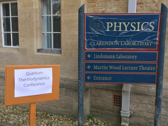
I recently had the pleasure of contributing to the general well-being of my academic colleagues by helping to co-organize (with Andrew Childs, Ignacio Cirac, and Umesh Vazirani) a 2-month long program on “Challenges in Quantum Computation” at the Simons Institute in Berkeley. In this post I report on the program and describe one of the highlights discussed during it: Mahadev’s very recent breakthrough on classical verification of quantum computation.

Challenges in Quantum Computation

The Simons Institute has been in place on the UC Berkeley campus since the Fall of 2013, and in fact one of their first programs was on “Quantum Hamiltonian Complexity”, in Spring 2014 (see my account of one of the semester’s workshops here). Since then the institute has been hosting a pair of semester-long programs at a time, in all areas of theoretical computer science and neighboring fields. Our “summer cluster” had a slightly different flavor: shorter, smaller, it doubled up as the prelude to a full semester-long program scheduled for Spring 2020 (provisional title: The Quantum Wave in Computing, a title inspired from Umesh Vazirani’s recent tutorial at STOC’18 in Los Angeles) — (my interpretation of) the idea being that the ongoing surge in experimental capabilities supports a much broader overhaul of some of the central questions of computer science, from the more applied (such as, programming languages and compilers), to the most theoretical (such as, what complexity classes play the most central role).

This summer’s program hosted a couple dozen participants at a time. Some stayed for the full 2 months, while others visited for shorter times. The Simons Institute is a fantastic place for collaborative research. The three-story building is entirely devoted to us. There are pleasant yet not-too-comfortable shared offices, but the highlight is the two large communal rooms meant for organized and spontaneous discussion. Filled with whiteboards, bright daylight, comfy couches, a constant supply of tea, coffee, and cookies, and eager theorists!

After a couple weeks of settling down the program kicked off with an invigorating workshop. Our goal for the workshop was to frame the theoretical questions raised by the sudden jump in the capabilities of experimental quantum devices that we are all witnessing. There were talks describing progress in experiments (superconducting qubits, ion traps, and cold atoms were represented), suggesting applications for the new devices (from quantum simulation & quantum chemistry to quantum optimization and machine learning through “quantum supremacy” and randomness generation), and laying the theoretical framework for trustworthy interaction with the quantum devices (interactive proofs, testing, and verifiable delegation). We had an outstanding line-up of speakers. All talks (except the panel discussions, unfortunately) were recorded, and you can watch them here.

The workshop was followed by five additional weeks of “residency”, that allowed long-term participants to digest and develop the ideas presented during the workshop. In my experience these few additional weeks, right after the workshop, make all the difference. It is the same difference as between a quick conference call and a leisurely afternoon at the whiteboard: while the former may feel productive and bring the adrenaline levels up, the latter is more suited to in-depth exploration and unexpected discoveries.

There would be much to say about the ideas discussed during the workshop and following weeks. I will describe a single one of these ideas — in my opinion, one of the most outstanding ideas to have emerged at the interface of quantum computing and theoretical computer science in recent years! The result, “Classical Verification of Quantum Computations”, is by Urmila Mahadev, a Ph.D.~student at UC Berkeley (I think she just graduated). Urmila gave a wonderful talk on her result at the workshop, and I highly recommend watching the recorded video. In the remainder of this post I’ll provide an overview of the result. I also wrote a slightly more technical introduction that eager readers will find here.

A cryptographic leash on quantum systems

Mahadev’s result is already famous: announced on the blog of Scott Aaronson, it has earned her a long-standing 25$ prize, awarded for “solving the problem of proving the results of an arbitrary quantum computation to a classical skeptic”. Or, in complexity-theoretic linguo, for showing that “every language in the class BQP admits an interactive protocol where the prover is in BQP and the verifier is in BPP”. What does this mean?

Verifying quantum computations in the high complexity regime

On his blog Scott Aaronson traces the question back to a talk given by Daniel Gottesman in 2004. An eloquent formulation appears in a subsequent paper by Dorit Aharonov and Umesh Vazirani, aptly titled “Is Quantum Mechanics Falsifiable? A computational perspective on the foundations of Quantum Mechanics”.

Here is the problem. As readers of this blog are well aware, Feynman’s idea of a quantum computer, and the subsequent formalization by Bernstein and Vazirani of the Quantum Turing Machine, layed the theoretical foundation for the construction of computing devices whose inner functioning is based on the laws of quantum physics. Most readers also probably realize that we currently believe that these quantum devices will have the ability to efficiently solve computational problems (the class of which is denoted BQP) that are thought to be beyond the reach of classical computers (represented by the class BPP). A prominent example is factoring, but there are many others. The most elementary example is arguably Feynman’s original proposal: a quantum computer can be used to simulate the evolution of any quantum mechanical system “in real time”. In contrast, the best classical simulations available can take exponential time to converge even on concrete examples of practical interest. This places a computational impediment to scientific progress: the work of many physicists, chemists, and biologists, would be greatly sped up if only they could perform simulations at will.

So this hypothetical quantum device claims (or will likely claim) that it has the ability to efficiently solve computational problems for which there is no known efficient classical algorithm. Not only this but, as is widely believed in complexity-theoretic circles (a belief recently strenghtened by the proof of an oracle separation between BQP and PH by Tal and Raz), for some of these problems, even given the answer, there does not exist a classical proof that the answer is correct. The quantum device’s claim cannot be verified! This seems to place the future of science at the mercy of an ingenuous charlatan, with good enough design & marketing skills, that would convince us that it is providing the solution to exponentially complex problems by throwing stardust in our eyes. (Wait, did this happen already?)

Today is the most exciting time in quantum computing since the discovery of Shor’s algorithm for factoring: while we’re not quite ready to run that particular algorithm yet, experimental capabilities have ramped up to the point where we are just about to probe the “high-complexity” regime of quantum mechanics, by making predictions that cannot be emulated, or even verified, using the most powerful classical supercomputers available. What confidence will we have that the predictions have been obtained correctly? Note that this question is different from the question of testing the validity of the theory of quantum mechanics itself. The result presented here assumes the validity of quantum mechanics. What it offers is a method to test, assuming the correctness of quantum mechanics, that a device performs the calculation that it claims to have performed. If the device has supra-quantum powers, all bets are off. Even assuming the correctness of quantum mechanics, however, the device may, intentionally or not (e.g. due to faulty hardware), mislead the experimentalist. This is the scenario that Mahadev’s result aims to counter.

Interactive proofs

The first key idea is to use the power of interaction. The situation can be framed as follows: given a certain computation, such that a device (henceforth called “prover”) has the ability to perform the computation, but another entity, the classical physicist (henceforth called “verifier”) does not, is there a way for the verifier to extract the right answer from the prover with high confidence — given that the prover may not be trusted, and may attempt to use its superior computing power to mislead the verifier instead of performing the required computation?

The simplest scenario would be one where the verifier can execute the computation herself, and check the prover’s outcome. The second simplest scenario is one where the verifier cannot execute the computation, but there is a short proof that the prover can provide that allows her to fully certify the outcome. These two scenario correspond to problems in BPP and NP respectively; an example of the latter is factoring. As argued earlier, not all quantum computations (BQP) are believed to fall within these two classes. Both direct computation and proof verification are ruled out. What can we do? Use interaction!

The framework of interactive proofs originates in complexity theory in the 1990s. An interactive proof is a protocol through which a verifier (typically a computationally bounded entity, such as the physicist and her classical laptop) interacts with a more powerful, but generally untrusted, prover (such as the experimental quantum device). The goal of the protocol is for the verifier to certify the validity of a certain computational statement.

Here is a classical example (the expert — or impatient — reader may safely skip this). The example is for a problem that lies in co-NP, but is not believed to lie in NP. Suppose that both the verifier and prover have access to two graphs, ${G}$ and ${H}$ , such that the verifier wishes to raise an “ACCEPT” flag if and only if the two graphs are not isomorphic. In general this is a hard decision to make, because the verifier would have to check all possible mappings from one graph to the other, of which there are exponentially many. Here is how the verifier can extract the correct answer by interacting with a powerful, untrusted prover. First, the verifier flips a fair coin. If the coin comes up heads, she selects a random relabeling of the vertices of ${G}$ . If the coin comes up tail, she selects a random relabeling of the vertices of ${H}$ . The verifier then sends the relabeled graph to the prover, and asks the prover to guess which graph the verifier has hidden. If the prover provides the correct answer (easy to check), the verifier concludes that the graphs were not isomorphic. Otherwise, she concludes that they were isomorphic. It is not hard to see that, if the graphs are indeed not isomorphic, the prover always has a means to correctly identify the hidden graph, and convince the verifier to make the right decision. But if the graphs are isomorphic, then there is no way for the prover to distinguish the random relabelings (since the distributions obtained by randomly relabeling each graph are identical), and so the verifier makes the right decision with probability 1/2. Repeating the protocol a few times, with a different choice of relabeling each time, quickly drives the probability of making an error to ${0}$ .

A deep result from the 1990s exactly charaterizes the class of computational problems (languages) that a classical polynomial-time verifier can decide in this model: IP = PSPACE. In words, any problem whose solution can be found in polynomial space has an interactive proof in which the verifier only needs polynomial time. Now observe that PSPACE contains NP, and much more: in fact PSPACE contains BQP as well (and even QMA)! (See this nice recent article in Quanta for a gentle introduction to these complexity classes, and more.) Thus any problem that can be decided on a quantum computer can also be decided without a quantum computer, by interacting with a powerful entity, the prover, that can convince the verifier of the right answer without being able to induce her in error (in spite of the prover’s greater power).

Are we not done? We’re not! The problem is that the result PSPACE = IP, even when specialized to BQP, requires (for all we know) a prover whose power matches that of PSPACE (almost: see e.g. this recent result for a slighlty more efficient prover). And as much as our experimental quantum device inches towards the power of BQP, we certainly wouldn’t dare ask it to perform a PSPACE-hard computation. So even though in principle there do exist interactive proofs for BQP-complete languages, these interactive proofs require a prover whose computational power goes much beyond what we believe is physically achievable. But that’s useless (for us): back to square zero.

Interactive proofs with quantum provers

Prior to Mahadev’s result, a sequence of beautiful results in the late 2000’s introduced a clever extension of the model of interactive proofs by allowing the verifier to make use of a very limited quantum computer. For example, the verifier may have the ability to prepare single qubits in two possible bases of her choice, one qubit at a time, and send them to the prover. Or the verifier may have the ability to receive single qubits from the prover, one at a time, and measure them in one of two bases of her choice. In both cases it was shown that the verifier could combine such limited quantum capacity with the possibility to interact with a quantum polynomial-time prover to verify arbitrary polynomial-time quantum computation. The idea for the protocols crucially relied on the ability of the verifier to prepare qubits in a way that any deviation by the prover from the presecribed honest behavior would be detected (e.g. by encoding information in mutually unbiased bases unknown to the prover). For a decade the question remained open: can a completely classical verifier certify the computation performed by a quantum prover?

Mahadev’s result brings a positive resolution to this question. Mahadev describes a protocol with the following properties. First, as expected, for any quantum computation, there is a quantum prover that will convince the classical verifier of the right outcome for the computation. This property is called completeness of the protocol. Second, no prover can convince the classical verifier to accept a wrong outcome. This property is called soundness of the protocol. In Mahadev’s result the latter property comes with a twist: soundness holds provided the prover cannot break post-quantum cryptography. In contrast, the earlier results mentioned in the previous paragraph obtained protocols that were sound against an arbitrarily powerful prover. The additional cryptographic assumption gives Mahadev’s result a “win-win” flavor: either the protocol is sound, or someone in the quantum cloud has figured out how to break an increasingly standard cryptographic assumption (namely, post-quantum security of the Learning With Errors problem) — in all cases, a verified quantum feat!

In the remaining of the post I will give a high-level overview of Mahadev’s protocol and its analysis. For more detail, see the accompanying blog post.

The protocol is constructed in two steps. The first step builds on insights from works preceding this one. This step reduces the problem of verifying the outcome of an arbitrary quantum computation to a seemingly much simpler problem, that nevertheless encapsulates all the subtlety of the verification task. The problem is the following — in keeping with the terminology employed by Mahadev, I’ll call it the qubit commitment problem. Suppose that a prover claims to have prepared a single-qubit state of its choice; call it ${| \psi \rangle}$ ( ${| \psi \rangle}$ is not known to the verifier). Suppose the verifier challenges the prover for the outcome of a measurement performed on ${| \psi \rangle}$ , either in the computational basis (the eigenbasis of the Pauli Z), or in the Hadamard basis (the eigenbasis of the Pauli X). Which basis to use is the verifier’s choice, but of course only one basis can be asked. Does there exist a protocol that guarantees that, at the end of the protocol, the verifier will be able to produce a bit that matches the true outcome of a measurement of ${| \psi \rangle}$ in the chosen basis? (More precisely, it should be that the verifier’s final bit has the same distribution as the outcome of a measurement of ${| \psi \rangle}$ in the chosen basis.)

The reduction that accomplishes this first step combines Kitaev’s circuit-to-Hamiltonian construction with some gadgetry from perturbation theory, and I will not describe it here. An important property of the reduction is that it is ultimately sufficient that the verifier has the guarantee that the measurement outcomes she obtains in either case, computational or Hadamard, are consistent with measurement outcomes for the correct measurements performed on some quantum state. In principle the state does not need to be related to anything the prover does (though of course the analysis will eventually define that state from the prover), it only needs to exist. Specifically, we wish to rule out situations where e.g. the prover claims that both outcomes are deterministically “0”, a claim that would violate the uncertainty principle. (For the sake of the argument, let’s ignore that in the case of a single qubit the space of outcomes allowed by quantum mechanics can be explicitly mapped out — in the actual protocol, the prover commits to ${n}$ qubits, not just one.)

Committing to a qubit

The second step of the protocol construction introduces a key idea. In order to accomplish the sought-after commitment, the verifier is going to engage in an initial commitment phase with the prover. In this phase, the prover is required to provide classical information to the verifier, that “commits” it to a specific qubit. This committed qubit is the state on which the prover will later perform the measurement asked by the verifier. The classical information obtained in the commitment phase will bind the prover to reporting the correct outcome, for both of the verifier’s basis choice — or risk being caught cheating. bit_commit_cartoon

How does this work? Commitments to bits, or even qubits, are an old story in cryptography. The standard method for committing to a bit ${b}$ is based on the use of a one-way permutation ${f}$ , together with a hardcore predicate ${h}$ for ${f}$ (i.e.~an efficiently computable function ${h: \{0,1\}^n\rightarrow \{0,1\}}$ such that given ${f(x)}$ , it is hard to predict ${h(x)}$ ). The construction goes as follows. The committer selects a uniformly random string ${r}$ and sends ${(y,m)=(f(r),h(r)\oplus b)}$ . To unveil the commitment ${b}$ , it is enough to reveal a string ${r}$ such that ${f(r)=y}$ ; the receiver can then compute ${h(r)}$ and decode ${b=h(r)\oplus m}$ . The point is that since ${f}$ is a permutation, the value ${y}$ uniquely “commits” the sender to an ${r}$ , and thus to a ${b}$ ; however, given ${y=f(r)}$ for an unknown ${r}$ the hardcore predicate ${h(r)}$ looks uniformly random, thus ${(y,m)}$ reveals no information about ${b}$ to the receiver.

What is new in Mahadev’s scheme is not only that the commitment is to a qubit, instead of a bit, but even more importabtly that the commitment is provided by classical information, which is necessary to obtain a classical protocol. (Commitments to qubits, using qubits, can be obtained by combining the quantum one-time pad with the commitment scheme described above.) To explain how this is achieved we’ll need a slightly more advanced crypographic primitive: a pair of injective trapdoor one-way functions ${f_0,f_1:\{0,1\}^n\rightarrow\{0,1\}^n}$ . This means that it is easy to evaluate both functions on any input, but that given a value ${y}$ in their common range, it is hard to find a preimage of ${y}$ under either function — except if one is given the trapdoor information. (Note that this is an over-simplification of the actual primitive used by Mahadev, which has additional properties, including that of being “claw-free”.)

The commitment phase of the protocol works as follows. Starting from a state ${| \psi \rangle=\alpha| 0 \rangle+\beta| 1 \rangle}$ of its choice, the prover is supposed to perform the following steps. First, the prover creates a uniform superposition over the common domain of ${f_0}$ and ${f_1}$ . Then it evaluates either function, ${f_0}$ or ${f_1}$ , in an additional register, by controlling on the qubit of ${| \psi \rangle}$ . Finally, the prover measures the register that contains the image of ${f_0}$ or ${f_1}$ . This achieves the following sequence of transformations:

$\displaystyle \begin{array}{rcl} \alpha| 0 \rangle+\beta| 1 \rangle &\mapsto& (\alpha| 0 \rangle + \beta| 1 \rangle) \otimes \Big(2^{-n/2} \sum_{x\in\{0,1\}^n} | x \rangle\Big) \\ &\mapsto & 2^{-n/2} \sum_x \alpha | 0 \rangle| x \rangle| f_0(x) \rangle + \beta | 1 \rangle| f_1(x) \rangle\\ &\mapsto & \big(\alpha| 0 \rangle| x_0 \rangle+\beta| 1 \rangle| x_1 \rangle\big)| y \rangle\;, \end{array}$

where ${y\in\{0,1\}^n}$ is the measured image. The string ${y}$ is called the prover’s commitment string. It is required to report it to the verifier.

In what sense is ${y}$ a commitment to the state ${| \psi \rangle}$ ? The key point is that, once it has measured ${y}$ , the prover has “lost control” over its qubit — it has effectively handed over that control to the verifier. For example, the prover no longer has the ability to perform an arbitrary rotation on its qubit. Why? The prover knows ${y}$ (it had to report it to the verifier) but not ${x_0}$ and ${x_1}$ (this is the claw-free assumption on the pair ${(f_0,f_1)}$ ). What this means — though of course it has to be shown — is that the prover can no longer recover the state ${| \psi \rangle}$ ! It does not have the ability to “uncompute” ${x_0}$ and ${x_1}$ . Thus the qubit has been “set in cryptographic stone”. In contrast, the verifier can use the trapdoor information to recover ${x_0}$ and ${x_1}$ . This gives her extra leverage on the prover. This asymmetry, introduced by cryptography, is what eventually allows the verifier to extract a truthful measurement outcome from the prover (or detect lying).

It is such a wonderful idea! It stuns me every time Urmila explains it. Proving it is of course rather delicate. In this post I make an attempt at going into the idea in a little more depth. The best resource remains Urmila’s paper, as well as her talk at the Simons Institute.

Open questions

What is great about this result is not that it closes a decades-old open question, but that by introducing a truly novel idea it opens up a whole new field of investigation. Some of the ideas that led to the result were already fleshed out by Mahadev in her work on homomorphic encryption for quantum circuits, and I expect many more results to continue building on these ideas.

An obvious outstanding question is whether the cryptography is needed at all: could there be a scheme achieving the same result as Mahadev’s, but without computational assumptions on the prover? It is known that if such a scheme exists, it is unlikely to have the property of being blind, meaning that the prover learns nothing about the computation that the verifier wishes it to execute (aside from an upper bound on its length); see this paper for “implausibility” results in this direction. Mahadev’s protocol relies on “post-hoc” verification, and is not blind. Urmila points out that it is likely the protocol could be made blind by composing it with her protocol for homomorphic encryption. Could there be a different protocol, that would not go through post-hoc verification, but instead directly guide the prover through the evaluation of a universal circuit on an encrypted input, gate by gate, as did some previous works?

So long, and thanks for all the Fourier transforms

Posted on July 29, 2018 by Nicole Yunger Halpern

The air conditioning in Caltech’s Annenberg Center for Information Science and Technology broke this July. Pasadena reached 87°F on the fourth, but my office missed the memo. The thermostat read 62°.

Hyperactive air conditioning suits a thermodynamicist’s office as jittery wifi suits an electrical-engineering building. Thermodynamicists call air conditioners “heat pumps.” A heat pump funnels heat—the energy of random motion—from cooler bodies to hotter. Heat flows spontaneously only from hot to cold on average, according to the Second Law of Thermodynamics. Pumping heat against its inclination costs work, organized energy drawn from a reliable source.

Reliable sources include batteries, coiled springs, and ACME anvils hoisted into the air. Batteries have chemical energy that power electric fans. ACME anvils have gravitational potential energy that splat coyotes.

I hoisted binder after binder onto my desk this July. The binders felt like understudies for ACME anvils, bulging with papers. They contained notes I’d written, and articles I’d read, for research throughout the past five years. My Caltech sojourn was switching off its lights and drawing its shutters. A control theorist was inheriting my desk. I had to move my possessions to an office downstairs, where I’d moonlight until quitting town.

Quitting town.

I hadn’t expected to feel at home in southern California, after stints in New and old England. But research and researchers drew me to California and then hooked me. Caltech’s Institute for Quantum Information and Matter (IQIM) has provided an intellectual home, colleagues-cum-friends, and a base from which to branch out to other scholars and institutions.

The IQIM has provided also the liberty to deck out my research program as a college dorm room with posters—according to my tastes, values, and exuberances. My thesis demanded the title “Quantum steampunk: Quantum information, thermodynamics, their intersection, and applications thereof across physics.” I began developing the concept of quantum steampunk on this blog. Writing a manifesto for the concept, in the thesis’s introduction, proved a delight:

The steampunk movement has invaded literature, film, and art over the past three decades. Futuristic technologies mingle, in steampunk works, with Victorian and wild-west settings. Top hats, nascent factories, and grimy cities counterbalance time machines, airships, and automata. The genre arguably originated in 1895, with the H.G. Wells novel The Time Machine. Recent steampunk books include the best-selling The Invention of Hugo Cabret; films include the major motion picture Wild Wild West; and artwork ranges from painting to jewelry to sculpture.

Steampunk captures the romanticism of fusing the old with the cutting-edge. Technologies proliferated during the Victorian era: locomotives, Charles Babbage’s analytical engine, factories, and more. Innovation facilitated exploration. Add time machines, and the spirit of adventure sweeps you away. Little wonder that fans flock to steampunk conventions, decked out in overcoats, cravats, and goggles.

What steampunk fans dream, quantum-information thermodynamicists live.

Thermodynamics budded during the late 1800s, when steam engines drove the Industrial Revolution. Sadi Carnot, Ludwig Boltzmann, and other thinkers wondered how efficiently engines could operate. Their practical questions led to fundamental insights—about why time flows; how much one can know about a physical system; and how simple macroscopic properties, like temperature, can capture complex behaviors, like collisions by steam particles. An idealization of steam—the classical ideal gas—exemplifies the conventional thermodynamic system. Such systems contain many particles, behave classically, and are often assumed to remain in equilibrium.

But thermodynamic concepts—such as heat, work, and equilibrium—characterize small scales, quantum systems, and out-of-equilibrium processes. Today’s experimentalists probe these settings, stretching single DNA strands with optical tweezers [4], cooling superconducting qubits to build quantum computers [5, 6], and extracting work from single-electron boxes [7]. These settings demand reconciliation with 19th-century thermodynamics. We need a toolkit for fusing the old with the new.

Quantum information (QI) theory provides such a toolkit. Quantum phenomena serve as resources for processing information in ways impossible with classical systems. Quantum computers can solve certain computationally difficult problems quickly; quantum teleportation transmits information as telephones cannot; quantum cryptography secures messages; and quantum metrology centers on high- precision measurements. These applications rely on entanglement (strong correlations between quantum systems), disturbances by measurements, quantum uncertainty, and discreteness.

Technological promise has driven fundamental insights, as in thermodynamics. QI theory has blossomed into a mathematical toolkit that includes entropies, uncertainty relations, and resource theories. These tools are reshaping fundamental science, in applications across physics, computer science, and chemistry.

QI is being used to update thermodynamics, in the field of quantum thermodynamics (QT) [8, 9]. QT features entropies suited to small scales; quantum engines; the roles of coherence in thermalization and transport; and the transduction of information into work, à la Maxwell’s demon [10].

This thesis (i) contributes to the theory of QI thermodynamics and (ii) applies the theory, as a toolkit, across physics. Spheres touched on include atomic, molecular, and optical (AMO) physics; nonequilibrium statistical mechanics; condensed matter; chemistry; and high-energy physics. I propose the name quantum steampunk for this program…

Never did I anticipate, in college, that a PhD could reflect my identity and style. I feared losing myself and my perspective in a subproblem of a subproblem of a subproblem. But I found myself blessed with the chance to name the aesthetic that’s guided my work, the scent I’ve unconsciously followed from book to class to research project to conversation, to paper, since…middle school, come to think of it. I’m grateful for that opportunity.

Whump, went my quantum-engine binder on my desk. I’d stuck an address label, pointing to Annenberg, to the binder. If the binder walked away, whoever found it would know where it belonged. Scratching at the label with a fingernail failed to budge the sticker. I stuck a label addressed to Cambridge, Massachusetts alongside the Pasadena address.

I’m grateful to be joining Harvard as an ITAMP (Institute for Theoretical Atomic, Molecular, and Optical Physics) Postdoctoral Fellow. You’ll be able to catch me in Harvard’s physics department, in ITAMP, or at MIT, starting this September.

While hunting for a Cambridge apartment, I skyped with potential roommates. I’d inquire about locations, about landlords and landladies, about tidiness, and about heating. The heating system’s pretty old, most tenants would admit. We keep the temperature between 60 and 65 degrees, to keep costs down. I’d nod and extol the layering of sweaters, but I shivered inside.

One tenant surprised me. The heating…works too well, she said. It’s pretty warm, to tell the truth. I thought about heat pumps and quantum engines, about picnics in the Pasadena sunshine, about the Julys I’d enjoyed while the world around me had sweated. Within an hour, I’d committed to sharing the apartment.

Some of you have asked whether I’ll continue blogging for Quantum Frontiers. Yes: Extricating me from the IQIM requires more than 3,000 miles.

See you in Cambridge.

With apologies to Douglas Adams.

The World Cup from a Quantum Perspective

Posted on July 2, 2018 by Johannes Bausch

Two weeks into the Football World Cup and the group stages are over: 16 teams have gone home, leaving the top 16 teams to contend the knock-out stages. Those fans who enjoy a bet will be poring over the odds in search of a bargain—a mis-calculation on the part of the bookmakers. Is now the time to back Ronaldo for the golden boot, whilst Harry Kane dominates the headlines and sports betting markets? Will the hosts Russia continue to defy lowly pre-tournament expectations and make the semi-finals? Are France about to emerge from an unconvincing start to the tournament and blossom as clear front-runners?

But, whilst for most the sports betting markets may lead to the enhanced enjoyment of the tournament that a bet can bring (as well as the possibility of making a little money), for others they represent a window into the fascinating world of sports statistics. A fascination that can be captured by the simple question: how do they set the odds?

Suppose that a bookmaker has in their possession a list of outcome probabilities for matches between each pair of national football teams in the world and wants to predict the overall winner. There are 32768 possible ways for the tournament knock-out rounds to pan-out—a large, but not insurmountable number of iterations by modern computational standards.

However, if the bookmaker instead considers the tennis grand-slams, with 128 competitors in the first round, then there are a colossal 1.7 × 10³⁸ permutations. Indeed, in a knock-out format there are 2^n-1 permutations, where n is the number of entrants. And for those of a certain mindset, this exponentially growing space immediately raises the question of whether a quantum algorithm can yield a speed-up for the related prediction tasks.

A Tiny Cup

The immediate question which we want to answer here is, perhaps, who will win the World Cup. We will walk through the idea on the blackboard first, and then implement it as a quantum algorithm—which, hopefully, will give some insight into how and where quantum computers can outperform classical ones, for this particular way of answering the question.

Let us take a toy setup with four teams A, B, C and D;
the knockout stage starts with a game A vs. B, and C vs. D.
Whoever wins each game will play against each other, so here we have four possible final games: A vs. C, A vs. D, B vs. C, or B vs. D.
Let’s denote by p(X, Y) the probability that X wins when playing against Y.

The likelihood of A winning the cup is then simply given by

p(A, B) × ( p(C, D) × p(A, C) + p(D, C) × p(A, D) ),

i.e. the probability that A wins against B, times the probabilities of A winning against C in case C won against D, plus the probability of A winning against D in case D won.

How can we obtain the same quantity with a quantum algorithm?

First, we set up our Hilbert space so that it can represent all possible Cup scenarios.
Since we have four teams, we need a four-dimensional quantum system as our smallest storage unit—we commonly call those qudits as generalizations of a qubit, which having dimension 2 would be fit to store two teams only (we can always “embed” a qudit into a few qubits of the same dimension.

Remember: k qubits have dimension 2^k, so we could also store the qudit as two qubits).
If we write $|A\rangle$ , this simply stands for a qudit representing team A; if we write $|A\rangle |B\rangle$ , then we have a state representing two teams.

To represent a full knockout tree, we follow the same logic: Take four qudits for the initial draw; add two qudits for the winners of the first two matches, and one qudit for the final winner.

For instance, one possible knockout scenario would be

$|\text{Game 1}\rangle = \underbrace{|A\rangle |B\rangle |C\rangle |D\rangle}_\text{Initial Draw} \ \underbrace{|A\rangle |D\rangle}_\text{Finals} \ |D\rangle.$

The probability associated with Game 1 is then precisely p(A, B) × p(D, C) × p(D, A).

Here is where quantum computing comes in.

Starting from an initial state $|A\rangle |B\rangle |C\rangle |D\rangle$ , we create two new slots in a superposition over all possible match outcomes, weighted by the square-root of their probabilities (which we call q instead of p):

$\begin{aligned} |\text{Step 1}\rangle = |A\rangle |B\rangle |C\rangle |D\rangle \big(\ \ &\text{q(A, B)q(C, D)} \,|A\rangle\ |C\rangle +\\ &\text{q(A, B)q(D, C)} \,|A\rangle\ |D\rangle +\\ &\text{q(B, A)q(C, D)} \,|B\rangle\ |C\rangle +\\ &\text{q(B, A)q(D, C)} \,|B\rangle\ |D\rangle\ \big). \end{aligned}$

So you can tell me who wins the World Cup?

Yes. Or well, probably. We find out by measuring the rightmost qudit.
As we know, the probability of obtaining a certain measurement outcome, say A, will then be determined by the square of the weights in front of the measured state; since we put in the square-roots initially we recover the original probabilities. Neat!

And since there are two possible game trees that lead to a victory of A, we have to sum them up—and we get precisely the probability we calculated by hand above. This means the team that is most likely to win will be the most likely measurement outcome.

So what about the World Cup? We have 16 teams; one team can thus be stored in four qubits. The knockout tree has 31 vertices, and a naive implementation can be done on a quantum computer with 124 qubits. Of course we are only a bit naive, so we can simulate this quantum computer on a classical one and obtain the following winning probabilities:

0.194	Brazil
0.168	Spain
0.119	France
0.092	Belgium
0.082	Argentina
0.075	England
0.049	Croatia
0.041	Colombia
0.04	Portugal
0.032	Uruguay
0.031	Russia
0.022	Switzerland
0.019	Denmark
0.018	Sweden
0.012	Mexico
0.006	Japan

It is worth noting that all operations we described can be implemented efficiently with a quantum computer, and the number of required qubits is quite small; for the four teams, we could get away with seven qudits, or fourteen qubits (and we could even save some, by ignoring the first four qudits which are always the same).

So for this particular algorithm there is an exponential speedup over its non-probabilistic classical counterpart: as mentioned, one would have to iterate over all trees; tedious for the World Cup, practically impossible for tennis. However…

Classical vs. Quantum

Does using a quantum algorithm give us a speedup for this task? Here, the answer is no; one could obtain similar results in comparable time using probabilistic methods, for instance, by doing Monte Carlo sampling.

But there are several interesting related questions that we could ask for which there might be a quantum advantage.

For some team A, we can easily create a state that has all game trees in superposition that lead to a victory of A—even weighting them using their respective probabilities.
Given this state as a resource, we can think of questions like “which game tree is most likely, given that we fix A and B as semifinalists”, or “which team should A play in the knockout stages to maximize the probability that B wins the tournament”.

Or, more controversially: can we optimize the winning chances for some team by rearranging the initial draw?

Some questions like these lend themselves to applying Grover search, for which there is a known speedup over classical computers. To inquire deeper into the utility of quantum algorithms, we need to invent the right kind of question to ask of this state.

Let us think of one more toy example. Being part physicists, we assume cows are spheres—so we might as well also assume that if A is likely to win a match against B, it always wins—even if the probability is only 51%. Let’s call this exciting sport “deterministic football”. For a set of teams playing a tournament of deterministic football, does there exist a winning initial draw for every team?

This becomes an especially interesting question in cases where there is a non-trivial cyclic relation between the teams’ abilities, a simple example being: A always beats B, B always beats C, and C always beats A. For example, if this problem turns out to be NP-hard, then it would be reasonable to expect that the quadratic improvement achieved by quantum search is the best we can hope for in using a quantum algorithm for the task of finding a winning initial draw for a chosen team—at least for deterministic football (phew).

To the finals and beyond

World Cup time is an exciting time: whatever the question, we are essentially dealing with binary trees, and making predictions can be translated into finding partitions or cuts that satisfy certain properties defined through a function of the edge weights (here the pairwise winning probabilities). We hope this quantum take on classical bookmaking might point us in the direction of new and interesting applications for quantum algorithms.

Hopefully a good bargain!

(Written with Steven Herbert and Sathyawageeswar Subramanian)

What’s the worst that could happen?

Posted on June 24, 2018 by Nicole Yunger Halpern

The archaeologist Howard Carter discovered Tutankhamun’s burial site in 1922. No other Egyptian pharaoh’s tomb had survived mostly intact until the modern era. Gold and glass and faience, statues and pendants and chariots, had evaded looting. The discovery would revolutionize the world’s understanding of, and enthusiasm for, ancient Egypt.

First, the artifacts had to leave the tomb.

Tutankhamun lay in three coffins nested like matryoshka dolls. Carter describes the nesting in his book The Tomb of Tutankhamen. Lifting the middle coffin from the outer coffin raised his blood pressure:

Everything may seem to be going well until suddenly, in the crisis of the process, you hear a crack—little pieces of surface ornament fall. Your nerves are at an almost painful tension. What is happening? All available room in the narrow space is crowded by your men. What action is needed to avert a catastrophe?

In other words, “What’s the worst that could happen?”

Collaborators and I asked that question in a paper published last month. We had in mind less Egyptology than thermodynamics and information theory. But never mind the distinction; you’re reading Quantum Frontiers! Let’s mix the fields like flour and oil in a Biblical grain offering.

Carter’s team had trouble separating the coffins: Ancient Egyptian priests (presumably) had poured fluid atop the innermost, solid-gold coffin. The fluid had congealed into a brown gunk, gluing the gold coffin to the bottom of the middle coffin. Removing the gold coffin required work—thermodynamic work.

Work consists of “well-ordered” energy usable in tasks like levering coffins out of sarcophagi and motoring artifacts from Egypt’s Valley of the Kings toward Cairo. We can model the gunk as a spring, one end of which was fixed to the gold coffin and one end of which was fixed to the middle coffin. The work $W$ required to stretch a spring depends on the spring’s stiffness (the gunk’s viscosity) and on the distance stretched through.

$W$ depends also on details: How many air molecules struck the gold coffin from above, opposing the team’s effort? How quickly did Carter’s team pull? Had the gunk above Tuankhamun’s nose settled into a hump or spread out? How about the gunk above Tutankhamun’s left eye socket? Such details barely impact the work required to open a 6.15-foot-long coffin. But air molecules would strongly impact $W$ if Tutankhamun measured a few nanometers in length. So imagine Egyptian matryoshka dolls as long as stubs of DNA.

Imagine that Carter found one million sets of these matryoshka dolls. Lifting a given set’s innermost coffin would require an amount $W$ of work that would vary from set of coffins to set of coffins. $W$ would satisfy fluctuation relations, equalities I’ve blogged about many times.

Fluctuation relations resemble the Second Law of Thermodynamics, which illuminates why time flows in just one direction. But fluctuation relations imply more-precise predictions about $W$ than the Second Law does.

Some predictions concern dissipated work: Carter’s team could avoid spending much work by opening the coffin infinitesimally slowly. Speeding up would heat the gunk, roil air molecules, and more. The heating and roiling would cost extra work, called dissipated work, denoted by $W_{\rm diss}$ .

Suppose that Carter’s team has chosen a lid-opening speed $v$ . Consider the greatest $W_{\rm diss}$ that the team might have to waste on any nanoscale coffin. $W_{\rm diss}^{\rm worst}$ is proportional to each of three information-theoretic quantities, my coauthors and I proved.

For experts: Each information-theoretic quantity is an order-infinity Rényi divergence $D_\infty ( X || Y)$ . The Rényi divergences generalize the relative entropy $D ( X || Y )$ . $D$ quantifies how efficiently one can distinguish between probability distributions, or quantum states, $X$ and $Y$ on average. The average is over many runs of a guessing game.

Imagine the worst possible run, which offers the lowest odds of guessing correctly. $D_\infty$ quantifies your likelihood of winning. We related $W_{\rm diss}^{\rm worst}$ to a $D_\infty$ between two statistical-mechanical phase-space distributions (when we described classical systems), to a $D_\infty$ between two quantum states (when we described quantum systems), and to a $D_\infty$ between two probability distributions over work quantities $W$ (when we described systems quantum and classical).

The worst case marks an extreme. How do the extremes consistent with physical law look? As though they’ve escaped from a mythologist’s daydream.

In an archaeologist’s worst case, arriving at home in the evening could lead to the following conversation:

“How was your day, honey?”

“The worst possible.”

“What happened?”

“I accidentally eviscerated a 3.5-thousand-year-old artifact—the most valuable, best-preserved, most information-rich, most lavishly wrought ancient Egyptian coffin that existed yesterday.”

Suppose that the archaeologist lived with a physicist. My group (guided by a high-energy physicist) realized that the conversation could continue as follows:

“And how was your day?”

“Also the worst possible.”

“What happened?”

“I created a black hole.”

General relativity and high-energy physics have begun breeding with quantum information and thermodynamics. The offspring bear extremes like few other systems imaginable. I wonder what our results would have to say about those offspring.

National Geographic reprinted Carter’s The Tomb of Tutankhamen in its “Adventure Classics” series. The series title fits Tomb as a mummy’s bandages fit the mummy. Carter’s narrative stretches from Egypt’s New Kingdom (of 3.5 thousand years ago) through the five-year hunt for the tomb (almost fruitless until the final season), to a water boy’s discovery of steps into the tomb, to the unsealing of the burial chamber, to the confrontation of Tutankhamun’s mummy.

Carter’s book guided me better than any audio guide could have at the California Science Center. The center is hosting the exhibition “King Tut: Treasures of the Golden Pharaoh.” After debuting in Los Angeles, the exhibition will tour the world. The tour showcases 150 artifacts from Tutankhamun’s tomb.

Those artifacts drove me to my desk—to my physics—as soon as I returned home from the museum. Tutankhamun’s tomb, Carter argues in his book, ranks amongst the 20th century’s most important scientific discoveries. I’d seen a smidgeon of the magnificence that Carter’s team— with perseverance, ingenuity, meticulousness, and buckets of sweat shed in Egypt’s heat—had discovered. I don’t expect to discover anything a tenth as magnificent. But how can a young scientist resist trying?

People say, “Prepare for the worst. Hope for the best.” I prefer “Calculate the worst. Hope and strive for a Tutankhamun.”

Postscript: Carter’s team failed to unglue the gold coffin by just “stretching” the gunky “spring.” The team resorted to heat, a thermodynamic quantity alternative to work: The team flipped the middle coffin upside-down above a heat lamp. The lamp raised the temperature to 932°F, melting the goo. The melting, with more work, caused the gold coffin to plop out of the middle coffin.

Catching up with the quantum-thermo crowd

Posted on April 15, 2018 by Nicole Yunger Halpern

You have four hours to tour Oxford University.

What will you visit? The Ashmolean Museum, home to da Vinci drawings, samurai armor, and Egyptian mummies? The Bodleian, one of Europe’s oldest libraries? Turf Tavern, where former president Bill Clinton reportedly “didn’t inhale” marijuana?

Felix Binder showed us a cemetery.

Of course he showed us a cemetery. We were at a thermodynamics conference.

The Fifth Quantum Thermodynamics Conference took place in the City of Dreaming Spires.¹Participants enthused about energy, information, engines, and the flow of time. About 160 scientists attended—roughly 60 more than attended the first conference, co-organizer Janet Anders estimated.

Weak measurements and quasiprobability distributions were trending. The news delighted me, Quantum Frontiers regulars won’t be surprised to hear.

Measurements disturb quantum systems, as early-20th-century physicist Werner Heisenberg intuited. Measure a system’s position strongly, and you forfeit your ability to predict the outcomes of future momentum measurements. Weak measurements don’t disturb the system much. In exchange, weak measurements provide little information about the system. But you can recoup information by performing a weak measurement in each of many trials, then processing the outcomes.

Strong measurements lead to probability distributions: Imagine preparing a particle in some quantum state, then measuring its position strongly, in each of many trials. From the outcomes, you can infer a probability distribution $\{ p(x) \}$ , wherein $p(x)$ denotes the probability that the next trial will yield position $x$ .

Weak measurements lead analogously to quasiprobability distributions. Quasiprobabilities resemble probabilities but can misbehave: Probabilities are real numbers no less than zero. Quasiprobabilities can dip below zero and can assume nonreal values.

What relevance have weak measurements and quasiprobabilities to quantum thermodynamics? Thermodynamics involves work and heat. Work is energy harnessed to perform useful tasks, like propelling a train from London to Oxford. Heat is energy that jiggles systems randomly.

Quantum properties obscure the line between work and heat. (Here’s an illustration for experts: Consider an isolated quantum, such as a spin chain. Let $H(t)$ denote the Hamiltonian that evolves with the time $t \in [0, t_f]$ . Consider preparing the system in an energy eigenstate $| E_i(0) \rangle$ . This state has zero diagonal entropy: Measuring the energy yields $E_i(0)$ deterministically. Considering tuning $H(t)$ , as by changing a magnetic field. This change constitutes work, we learn in electrodynamics class. But if $H(t)$ changes quickly, the state can acquire weight on multiple energy eigenstates. The diagonal entropy rises. The system’s energetics have gained an unreliability characteristic of heat absorption. But the system has remained isolated from any heat bath. Work mimics heat.)

Quantum thermodynamicists have defined work in terms of a two-point measurement scheme: Initialize the quantum system, such as by letting heat flow between the system and a giant, fixed-temperature heat reservoir until the system equilibrates. Measure the system’s energy strongly, and call the outcome $E_i$ . Isolate the system from the reservoir. Tune the Hamiltonian, performing the quantum equivalent of propelling the London train up a hill. Measure the energy, and call the outcome $E_f$ .

Any change $\Delta E$ in a system’s energy comes from heat $Q$ and/or from work $W$ , by the First Law of Thermodynamics, $\Delta E = Q + W.$ Our system hasn’t exchanged energy with any heat reservoir between the measurements. So the energy change consists of work: $E_f - E_i =: W$ .

Imagine performing this protocol in each of many trials. Different trials will require different amounts $W$ of work. Upon recording the amounts, you can infer a distribution $\{ p(W) \}$ . $p(W)$ denotes the probability that the next trial will require an amount $W$ of work.

Measuring the system’s energy disturbs the system, squashing some of its quantum properties. (The measurement eliminates coherences, relative to the energy eigenbasis, from the state.) Quantum properties star in quantum thermodynamics. So the two-point measurement scheme doesn’t satisfy everyone.

Enter weak measurements. They can provide information about the system’s energy without disturbing the system much. Work probability distributions $\{ p(W) \}$ give way to quasiprobability distributions $\{ \tilde{p}(W) \}$ .

So propose Solinas and Gasparinetti, in these papers. Other quantum thermodynamicists apply weak measurements and quasiprobabilities differently.² I proposed applying them to characterize chaos, and the scrambling of quantum information in many-body systems, at the conference.³ Feel free to add your favorite applications to the “comments” section.

All the quantum ladies: The conference’s female participants gathered for dinner one conference night.

Wednesday afforded an afternoon for touring. Participants congregated at the college of conference co-organizer Felix Binder.³ His tour evoked, for me, the ghosts of thermo conferences past: One conference, at the University of Cambridge, had brought me to the grave of thermodynamicist Arthur Eddington. Another conference, about entropies in information theory, had convened near Canada’s Banff Cemetery. Felix’s tour began with St. Edmund Hall’s cemetery. Thermodynamics highlights equilibrium, a state in which large-scale properties—like temperature and pressure—remain constant. Some things never change.

With thanks to Felix, Janet, and the other coordinators for organizing the conference.

¹Oxford derives its nickname from an elegy by Matthew Arnold. Happy National Poetry Month!

²https://arxiv.org/abs/1508.00438, https://arxiv.org/abs/1610.04285,
https://arxiv.org/abs/1607.02404,
https://journals.aps.org/prl/abstract/10.1103/PhysRevLett.118.070601,
https://journals.aps.org/prl/abstract/10.1103/PhysRevLett.120.040602

³Michele Campisi joined me in introducing out-of-time-ordered correlators (OTOCs) into the quantum-thermo conference: He, with coauthor John Goold, combined OTOCs with the two-point measurement scheme.

³Oxford University contains 38 colleges, the epicenters of undergraduates’ social, dining, and housing experiences. Graduate students and postdoctoral scholars affiliate with colleges, and senior fellows—faculty members—govern the colleges.

Rock-paper-scissors, granite-clock-idea

Posted on March 18, 2018 by Nicole Yunger Halpern

I have a soft spot for lamassu. Ten-foot-tall statues of these winged bull-men guarded the entrances to ancient Assyrian palaces. Show me lamassu, or apkallu—human-shaped winged deities—or other reliefs from the Neo-Assyrian capital of Nineveh, and you’ll have trouble showing me the door.

Assyrian art fills a gallery in London’s British Museum. Lamassu flank the gallery’s entrance. Carvings fill the interior: depictions of soldiers attacking, captives trudging, and kings hunting lions. The artwork’s vastness, its endurance, and the contact with a three-thousand-year-old civilization floor me. I tore myself away as the museum closed one Sunday night.

I visited the British Museum the night before visiting Jonathan Oppenheim’s research group at University College London (UCL). Jonathan combines quantum information theory with thermodynamics. He and others co-invented thermodynamic resource theories (TRTs), which Quantum Frontiers regulars will know of. TRTs are quantum-information-theoretic models for systems that exchange energy with their environments.

Energy is conjugate to time: Hamiltonians, mathematical objects that represent energy, represent also translations through time. We measure time with clocks. Little wonder that one can study quantum clocks using a model for energy exchanges.

Mischa Woods, Ralph Silva, and Jonathan used a resource theory to design an autonomous quantum clock. “Autonomous” means that the clock contains all the parts it needs to operate, needs no periodic winding-up, etc. When might we want an autonomous clock? When building quantum devices that operate independently of classical engineers. Or when performing a quantum computation: Computers must perform logical gates at specific times.

Wolfgang Pauli and others studied quantum clocks, the authors recall. How, Pauli asked, would an ideal clock look? Its Hamiltonian, $\hat{H}_{\rm C}$ , would have eigenstates $| E \rangle$ . The labels $E$ denote possible amounts of energy.

The Hamiltonian would be conjugate to a “time operator” $\hat{t}$ . Let $| \theta \rangle$ denote an eigenstate of $\hat{t}$ . This “time state” would equal an even superposition over the $| E \rangle$ ’s. The clock would occupy the state $| \theta \rangle$ at time $t_\theta$ .

Imagine measuring the clock, to learn the time, or controlling another system with the clock. The interaction would disturb the clock, changing the clock’s state. The disturbance wouldn’t mar the clock’s timekeeping, if the clock were ideal. What would enable an ideal clock to withstand the disturbances? The ability to have any amount of energy: $E$ must stretch from $- \infty$ to $\infty$ . Such clocks can’t exist.

Approximations to them can. Mischa, Ralph, and Jonathan designed a finite-size clock, then characterized how accurately the clock mimics the ideal. (Experts: The clock corresponds to a Hilbert space of finite dimensionality $d$ . The clock begins in a Gaussian state that peaks at one time state $| \theta \rangle$ . The finite-width Gaussian offers more stability than a clock state.)

Disturbances degrade our ability to distinguish instants by measuring the clock. Imagine gazing at a kitchen clock through blurry lenses: You couldn’t distinguish 6:00 from 5:59 or 6:01. Disturbances also hinder the clock’s ability to implement processes, such as gates in a computation, at desired instants.

Mischa & co. quantified these degradations. The errors made by the clock, they found, decay inverse-exponentially with the clock’s size: Grow the clock a little, and the errors shrink a lot.

Time has degraded the lamassu, but only a little. You can distinguish feathers in their wings and strands in their beards. People portray such artifacts as having “withstood the flow of time,” or “evaded,” or “resisted.” Such portrayals have never appealed to me. I prefer to think of the lamassu as surviving not because they clash with time, but because they harmonize with it. The prospect of harmonizing with time—whatever that means—has enticed me throughout my life. The prospect partially underlies my research into time—perhaps childishly, foolishly—I recognize if I remove my blurry lenses before gazing in the mirror.

The creation of lasting works, like lamassu, has enticed me throughout my life. I’ve scrapbooked, archived, and recorded, and tended memories as though they were Great-Grandma’s cookbook. Ancient civilizations began alluring me at age six, partially due to artifacts’ longevity. No wonder I study the second law of thermodynamics.

Yet doing theoretical physics makes no sense from another perspective. The ancient Egyptians sculpted granite, when they could afford it. Gudea, king of the ancient city-state of Lagash, immortalized himself in diorite. I fashion ideas, which lack substance. Imagine playing, rather than rock-paper-scissors, granite-diorite-idea. The idea wouldn’t stand a chance.

Would it? Because an idea lacks substance, it can manifest in many forms. Plato’s cave allegory has manifested as a story, as classroom lectures, on handwritten pages, on word processors and websites, in cartloads of novels, in the film The Matrix, in one of the four most memorable advertisements I received from colleges as a high-school junior, and elsewhere. Plato’s allegory has survived since about the fourth century BCE. King Ashurbanipal’s lion-hunt reliefs have survived for only about 200 years longer.

The lion-hunt reliefs—and lamassu—exude a grandness, a majesty that’s attracted me as their longevity has. The nature of time and the perfect clock have as much grandness. Leaving the British Museum’s Assyrian gallery at 6 PM one Sunday, I couldn’t have asked for a more fitting location, 24 hours later, than in a theoretical-physics conversation.

With thanks to Jonathan, to Álvaro Martín-Alhambra, and to Mischa for their hospitality at UCL; to Ada Cohen for the “Art history of ancient Egypt and the ancient Near East” course for which I’d been hankering for years; to my brother, for transmitting the ancient-civilizations bug; and to my parents, who fed the infection with museum visits.

Click here for a follow-up to the quantum-clock paper.

Fractons, for real?

Posted on February 16, 2018 by xiechen

“Fractons” is my favorite new toy (short for quantum many-body toy models). It has amazing functions that my old toys do not have; it is so new that there are tons of questions waiting to be addressed; it is perfectly situated at the interface between quantum information and condensed matter and has attracted a lot of interest and efforts from both sides; and it gives me excuses and new incentives to learn more math. I have been having a lot of fun playing with it in the last couple years and in the process, I had the great opportunity to work with some amazing collaborators: Han Ma and Mike Hermele at Boulder, Ethan Lake at MIT, Wilbur Shirley at Caltech, Kevin Slagle at U Toronto and Zhenghan Wang at Station Q. Together we have written a few papers on this subject, but I always felt there are more interesting stories and more excitement in me than what can be properly contained in scientific papers. Hence this blog post.

How I first learned about Fractons

Back in the early 2000s, a question that kept attracting and frustrating people in quantum information is how to build a quantum hard drive to store quantum information. This is of course a natural question to ask as quantum computing has been demonstrated to be possible, at least in theory, and experimental progress has shown great potential. It turned out, however, that the question is one of those deceptively enticing ones which are super easy to state, but extremely hard to answer. In a classical hard drive, information is stored using magnetism. Quantum information, instead of being just 0 and 1, is represented using superpositions of 0 and 1, and can be probed in non-commutative ways (that is, measuring along different directions can alter previous answers). To store quantum information, we need “magnetism” in all such non-commutative channels. But how can we do that?

At that time, some proposals had been made, but they either involve actively looking for and correcting errors throughout the time during which information is stored (which is something we never have to do with our classical hard drives) or going into four spatial dimensions. Reliable passive storage of quantum information seemed out of reach in the three-dimensional world we live in, even at the level of a proof of principle toy model!

Given all the previously failed attempts and without a clue about where else to look, this problem probably looked like a dead-end to many. But not to Jeongwan Haah, a fearless graduate student in Preskill’s group at IQIM at that time, who turned the problem from guesswork into a systematic computer search (over a constrained set of models). The result of the search surprised everyone. Jeongwan found a three-dimensional quantum spin model with physical properties that had never been seen before, making it a better quantum hard drive than any other model that we know of!

The model looks surprising not only to the quantum information community, but even more so to the condensed matter community. It is a strongly interacting quantum many-body model, a subject that has been under intense study in condensed matter physics. Yet it exhibits some very strange behaviors whose existence had not even been suspected. It is a condensed matter discovery made not from real materials in real experiments, but through computer search!

$fractal$

Excitations (stars) in Haah’s code live at the corner of a fractal.

In condensed matter systems, what we know can happen is that elementary excitations can come in the form of point particles – usually called quasi-particles – which can then move around and interact with other excitations. In Jeongwan’s model, now commonly referred to as Haah’s code, elementary excitations still come in the form of point particles, but they cannot freely move around. Instead, if they want to move, four of them have to coordinate with each other to move together, so that they stay at the vertices of a fractal shaped structure! The restricted motion of the quasi-particles leads to slower dynamics at low energy, making the model much better suited for the purpose of storing quantum information.

But how can something like this happen? This is the question that I want to yell out loud every time I read Jeongwan’s papers or listen to his talks. Leaving aside the motivation of building a quantum hard drive, this model presents a grand challenge to the theoretical framework we now have in condensed matter. All of our intuitions break down in predicting the behavior of this model; even some of the most basic assumptions and definitions do not apply.

The interactions in Haah’s code involve eight spins at a time (the eight Z’s and eight X’s in each cube).

I felt so uncomfortable and so excited at the same time because there was something out there that should be related to things I know, yet I totally did not understand how. And there was an even bigger problem. I was like a sick person going to a doctor but unable to pinpoint what was wrong. Something must have been wrong, but I didn’t know what that was and I didn’t know how to even begin to look for it. The model looked so weird. Interaction involved eight spins at a time; there was no obvious symmetry other than translation. Jeongwan, with his magic math power, worked out explicitly many of the amazing properties of the model, but that to me only added to the mystery. Where did all these strange properties coming from?

From the unfathomable to the seemingly approachable

I remained in this superposition of excited state and powerless state for several years, until Jeongwan moved to MIT and posted some papers with Sagar Vijay and Liang Fu in 2015 and 2016.

Interaction terms in a nicer looking fracton model.

In these papers, they listed several other models, which, similar to Haah’s code, contain quasi-particle excitations whose motion is constrained. The constraints are weaker and these models do not make good quantum hard drives, but they still represent new condensed matter phenomena. What’s nice about these models is that the form of interaction is more symmetric, takes a simpler form, or is similar to some other models we are familiar with. The quasi-particles do not need a fractal-shaped structure to move around, instead they move along a line, in a plane, or at the corner of a rectangle. In fact, as early as 2005 – six years before Haah’s code, Claudio Chamon at Boston University already proposed a model of this kind. Together with the previous fractal examples, these models are what’s now being referred to as the fracton models. If the original Haah’s code looks like an ET from beyond the milky way, these models at least seem to live somewhere in the solar system. So there must be something that we can do to understand them better!

Obviously, I was not the only one who felt this way. A flurry of papers appeared on these “fracton” models. People came at these models armed with their favorite tools in condensed matter, looking for an entry point to crack them open. The two approaches that I found most attractive was the coupled layer construction and the higher rank gauge theory, and I worked on these ideas together with Han Ma, Ethan Lake and Michael Hermele. Each approach comes from a different perspective and establishes a connection between fractons and physical models that we are familiar with. In the coupled layer construction, the connection is to the 2D discrete gauge theories, while in the higher rank approach it is to the 3D gauge theory of electromagnetism.

I was excited about these results. They each point to simple physical mechanisms underlying the existence of fractons in some particular models. By relating these models to things I already know, I feel a bit relieved. But deep down, I know that this is far from the complete story. Our understanding barely goes beyond the particular models discussed in the paper. In condensed matter, we spend a lot of time studying toy models; but toy models are not the end goal. Toy models are only meaningful if they represent some generic feature in a whole class of models. It is not clear at all to what extent this is the case for fractons.

Step zero: define “order”, define “topological order”

I gave a talk about these results at KITP last fall under the title “Fracton Topological Order”. It was actually too big a title because all we did was to study specific realizations of individual models and analyze their properties. To claim topological order, one needs to show much more. The word “order” refers to the common properties of a continuous range of models within the same phase. For example, crystalline order refers to the regular lattice organization of atoms in the solid phase within a continuous range of temperature and pressure. When the word “topological” is added in front of “order”, it signifies that such properties are usually directly related to the topology of the system. A prototypical example is the fractional quantum Hall system, whose ground state degeneracy is directly determined by the topology of the manifold the system lives in. For fractons, we are far from an understanding at this level. We cannot answer basic questions like what range of models form a phase, what is the order (the common properties of this whole range of models) characterizing each phase, and in what sense is the order topological. So, the title was more about what I hope will happen than what has already happened.

But it did lead to discussions that could make things happen. After my talk, Zhenghan Wang, a mathematician at Microsoft Station Q, said to me, “I would agree these fracton models are topological if you can show me how to define them on different three manifolds”. Of course! How can I claim anything related to topology if all I know is one model on a cubic lattice with periodic boundary condition? It is like claiming a linear relation between two quantities with only one data point.

But how to get more data points? Well, from the paper by Haah, Vijay and Fu, we knew how to define the model on cubic lattices. With periodic boundary conditions, the underlying manifold is a three torus. Is it possible to have a cubic lattice, or something similar, in other three manifolds as well? Usually, this kind of request would be too much to ask. But it turns out that if you whisper your wish to the right mathematician, even the craziest ones can come true. With insightful suggestions from Michael Freedman (the Fields medalist leading Station Q) and Zhenghan, and through the amazing work of Kevin Slagle (U Toronto) and Wilbur Shirley (Caltech), we found that if we make use of a structure called Total Foliation, one of the fracton models can be generalized to different kinds of three manifolds and we can see how the properties of the model are related to certain topological features of the manifold!

Foliation.

Foliation is the process of dividing a manifold into parallel planes. Total foliation is a set of three foliations which intersect each other in a transversal way. The xy, yz, and zx planes in a cubic lattice form a total foliation and similar constructions can be made for other three manifolds as well.

Things start to get technical from here, but the basic lesson we learned about some of the fracton models is that structural-wise, they pretty much look like an onion. Even though onions look like a three-dimensional object from the outside, they actually grow in a layered structure. Some of the properties of the fracton models are simply determined by the layers, and related

to the topology of the layers. Once we peel off all the layers, we find that for some, there is nothing left while for others, there is a nontrivial core. This observation allows us to better address the previous questions: we defined a fracton phase (one type of it) as models smoothly related to each other after adding or removing layers; the topological nature of the order is manifested in how the properties of the model are determined by the topology of the layers.

The onion structure is nice, because it allows us to reduce much of the story from 3D to 2D, where we understand things much better. It clarifies many of the weirdnesses of the fracton model we studied, and there is indication that it may apply to a much wider range of fracton models, so we have an exciting road ahead of us. On the other hand, it is also clear that the onion structure does not cover everything. In particular, it does not cover Haah’s code! Haah’s code cannot be built in a layered way and its properties are in a sense intrinsically three dimensional. So, after finishing this whole journey through the onion field, I will be back to staring at Haah’s code again and wondering what to do with it, like what I have been doing in the eight years since Jeongwan’s paper first came out. But maybe this time I will have some better ideas.

Machine learning the arXiv

Posted on November 29, 2017 by Evert van Nieuwenburg

Over the last year or so, the machine learning wave has really been sweeping through the field of condensed matter physics. Machine learning techniques have been applied to condensed matter physics before, but very sparsely and with little recognition. These days, I guess (partially) due to the general machine learning and AI hype, the amount of such studies skyrocketed (I admit to contributing to that..). I’ve been keeping track of this using the arXiv and Twitter (@Evert_v_N), but you should know about this website for getting an overview of the physics & machine learning papers: https://physicsml.github.io/pages/papers.html.

This effort of applying machine learning to physics is a serious attempt at trying to understand how such tools could be useful in a variety of ways. It isn’t very hard to get a neural network to learn ‘something’ from physics data, but it is really hard to find out what – and especially how – the network does that. That’s why toy cases such as the Ising model or the Kosterlitz-Thouless transition have been so important!

When you’re keeping track of machine learning and AI developments, you soon realize that there are examples out there of amazing feats. Being able to generate photo-realistic pictures given just a sentence. e.g. “a brown bird with golden speckles and red wings is sitting on a yellow flower with pointy petals”, is (I think..) pretty cool. I can’t help but wonder if we’ll get to a point where we can ask it to generate “the groundstate of the Heisenberg model on a Kagome lattice of 100×100”…

Another feat I want to mention, and the main motivation for this post, is that of being able to encode words as vectors. That doesn’t immediately seem like a big achievement, but it is once you want to have ‘similar’ words have ‘similar’ vectors. That is, you intuitively understand that Queen and King are very similar, but differ basically only in gender. Can we teach that to a computer (read: neural network) by just having it read some text? Turns out we can. The general encoding of words to vectors is aptly named ‘Word2Vec’, and some of the top algorithms that do that were introduced here (https://arxiv.org/abs/1301.3781) and here (https://arxiv.org/abs/1310.4546). The neat thing is that we can actually do arithmetics with these words encoded as vectors, so that the network learns (with no other input than text!):

King – Man + Woman = Queen
Paris – France + Italy = Rome

In that spirit, I wondered if we can achieve the same thing with physics jargon. Everyone knows, namely, that “electrons + two dimensions + magnetic field = Landau levels”. But is that clear from condensed matter titles?

Try it yourself

If you decide at this point that the rest of the blog is too long, at least have a look here: everthemore.pythonanywhere.com or skip to the last section. That website demonstrates the main point of this post. If that sparks your curiosity, read on!

This post is mainly for entertainment, and so a small disclaimer is in order: in all of the results below, I am sure things can be improved upon. Consider this a ‘proof of principle’. However, I would be thrilled to see what kind of trained models you can come up with yourself! So for that purpose, all of the code (plus some bonus content!) can be found on this github repository: https://github.com/everthemore/physics2vec.

Harvesting the arXiv

The perfect dataset for our endeavor can be found in the form of the arXiv. I’ve written a small script (see github repository) that harvests the titles of a given section from the arXiv. It also has options for getting the abstracts, but I’ll leave that for a separate investigation. Note that in principle we could also get the source-files of all of these papers, but doing that in bulk requires a payment; and getting them one by one will 1) take forever and 2) probably get us banned.

Collecting all this data of the physics:cond-mat subsection took right about 1.5 hours and resulted in 240737 titles and abstracts (I last ran this script on November 20^th, 2017). I’ve filtered them by year and month, and you can see the result in Fig.1 below. Seems like we have some catching up to do in 2017 still (although as the inset shows, we have nothing to fear. November is almost over, but we still have the ‘getting things done before x-mas’ rush coming up!).

Figure 1: The number of papers in the cond-mat arXiv section over the years. We’re behind, but the year isn’t over yet! (Data up to Nov 20th 2017)

Analyzing n-grams

After tidying up the titles (removing LaTeX, converting everything to lowercase, etc.), the next thing to do is to train a language model on finding n-grams. N-grams are basically fixed n-word expressions such as ‘cooper pair’ (bigram) or ‘metal insulator transition’ (trigram). This makes it easier to train a Word2Vec encoding, since these phrases are fixed and can be considered a single word. The python module we’ll use for Word2Vec is gensim (https://radimrehurek.com/gensim/), and it conveniently has phrase-detection built-in. The language model it builds reports back to us the n-grams it finds, and assigns them a score indicating how certain it is about them. Notice that this is not the same as how frequently it appears in the dataset. Hence an n-gram can appear fewer times than another, but have a higher certainty because it always appears in the same combination. For example, ‘de-haas-van-alphen’ appears less than, but is more certain than, ‘cooper-pair’, because ‘pair’ does not always come paired (pun intended) with ‘cooper’. I’ve analyzed up to 4-grams in the analysis below.

I can tell you’re curious by now to find out what some of the most certain n-grams in cond-mat are (again, these are not necessarily the most frequent), so here are some interesting findings:

The most certain n-grams are all surname combo’s, Affleck-Kennedy-Lieb-Tasaki being the number 1. Kugel-Khomskii is the most certain 2-name combo and Einstein-Podolksi-Rosen the most certain 3-name combo.
The first certain non-name n-gram is a ‘quartz tuning fork’, followed by a ‘superconducting coplanar waveguide resonator’. Who knew.
The bigram ‘phys. rev.’ and trigram ‘phys. rev. lett.’ are relatively high up in the confidence lists. These seem to come from the “Comment on […]”-titles on the arXiv.
I learned that there is such a thing as a Lefschetz thimble. I also learned that those things are called thimbles in English (we (in Holland) call them ‘finger-hats’!).

In terms of frequency however, which is probably more of interest to us, the most dominant n-grams are Two-dimensional, Quantum dot, Phase transition, Magnetic field, One dimensional and Bose-Einstein (in descending order). It seems 2D is still more popular than 1D, and all in all the top n-grams do a good job at ‘defining’ condensed matter physics. I’ll refer you to the github repository code if you want to see a full list! You’ll find there a piece of code that produces wordclouds from the dominant words and n-grams too, such as this one:

For fun though, before we finally get to the Word2Vec encoding, I’ve also kept track of all of these as a function of year, so that we can now turn to finding out which bigrams have been gaining the most popularity. The table below shows the top 5 n-grams for the period 2010 – 2016 (not including 2017) and for the period 2015 – Nov 20^th 2017.

2010-2016	2015 – November 20^th 2017
Spin liquids	Topological phases & transitions
Weyl semimetals	Spin chains
Topological phases & transitions	Machine learning
Surface states	Transition metal dichalcogenides
Transition metal dichalcogenides	Thermal transport
Many-body localization	Open quantum systems

Actually, the real number 5 in the left column was ‘Topological insulators’, but given number 3 I skipped it. Also, this top 5 includes a number 6 (!), which I just could not leave off given that everyone seems to have been working on MBL. If we really want to be early adopters though, taking only the last 1.8 years (2015 – now, Nov 20^th 2017) in the right column of the table shows some interesting newcomers. Surprisingly, many-body localization is not even in the top 20 anymore. Suffice it to say, if you have been working on anything topology-related, you have nothing to worry about. Machine learning is indeed gaining lots of attention, but we’ve yet to see if it doesn’t go the MBL-route (I certainly don’t hope so!). Quantum computing does not seem to be on the cond-mat radar, but I’m certain we would find that high up in the quant-ph arXiv section.

CondMat2Vec

Alright, finally time to use some actual neural networks for machine learning. As I started this post, what we’re about to do is try to train a network to encode/decode words into vectors, while simultaneously making sure that similar words (by meaning!) have similar vectors. Now that we have the n-grams, we want the Word2Vec algorithm to treat these as words by themselves (they are, after all, fixed combinations).

In the Word2Vec algorithm, we get to decide the length of the vectors that encode words ourselves. Larger vectors means more freedom in encoding words, but also makes it harder to learn similarity. In addition, we get to choose a window-size, indicating how many words the algorithm will look ahead to analyze relations between words. Both of these parameters are free for you to play with if you have a look at the source code repository. For the website everthemore.pythonanywhere.com, I’ve uploaded a size 100 with window-size 10 model, which I found to produce sensible results. Sensible here means “based on my expectations”, such as the previous example of “2D + electrons + magnetic field = Landau levels”. Let’s ask our network some questions.

First, as a simple check, let’s see what our encoding thinks some jargon is similar to:

Superconductor ~ Superconducting, Cuprate superconductor, Superconductivity, Layered superconductor, Unconventional superconductor, Superconducting gap, Cuprate, Weyl semimetal, …
Majorana ~ Majorana fermion, Majorana mode, Non-abelian, Zero-energy, braiding, topologically protected, …

It seems we could start to cluster words based on this. But the real test comes now, in the form of arithmetics. According to our network (I am listing the top two choices in some cases; the encoder outputs a list of similar vectors, ordered by similarity):

Majorana + Braiding = Non-Abelian
Electron + Hole = Exciton, Carrier
Spin + Magnetic field = Magnetization, Antiferromagnetic
Particle + Charge = Electron, Charged particle

And, sure enough:

2D + electrons + magnetic field = Landau level, Magnetoresistance oscillation

The above is just a small sample of the things I’ve tried. See the link in the try it yourself section above if you want to have a go. Not all of the examples work nicely. For example, neither lattice + wave nor lattice + excitation nor lattice + force seem to result in anything related to the word ‘phonon’. I would guess that increasing the window size will help remedy this problem. Even better probably would be to include abstracts!

Outlook

I could play with this for hours, and I’m sure that by including the abstracts and tweaking the vector size (plus some more parameters I haven’t even mentioned) one could optimize this more. Once we have an optimized model, we could start to cluster the vectors to define research fields, visualizing the relations between n-grams (both suggestions thanks to Thomas Vidick and John Preskill!), and many other things. This post has become rather long already however, and I will leave further investigation to a possible future post. I’d be very happy to incorporate anything cool you find yourselves though, so please let me know!

Gently yoking yin to yang

Posted on November 26, 2017 by Nicole Yunger Halpern

The architecture at the University of California, Berkeley mystified me. California Hall evokes a Spanish mission. The main library consists of white stone pillared by ionic columns. A sea-green building scintillates in the sunlight like a scarab. The buildings straddle the map of styles.

So do Berkeley’s quantum scientists, information-theory users, and statistical mechanics.

The chemists rove from abstract quantum information (QI) theory to experiments. Physicists experiment with superconducting qubits, trapped ions, and numerical simulations. Computer scientists invent algorithms for quantum computers to perform.

Few activities light me up more than bouncing from quantum group to info-theory group to stat-mech group, hunting commonalities. I was honored to bounce from group to group at Berkeley this September.

What a trampoline Berkeley has.

The groups fan out across campus and science, but I found compatibility. Including a collaboration that illuminated quantum incompatibility.

Quantum incompatibility originated in studies by Werner Heisenberg. He and colleagues cofounded quantum mechanics during the early 20th century. Measuring one property of a quantum system, Heisenberg intuited, can affect another property.

The most famous example involves position and momentum. Say that I hand you an electron. The electron occupies some quantum state represented by $| \Psi \rangle$ . Suppose that you measure the electron’s position. The measurement outputs one of many possible values $x$ (unless $| \Psi \rangle$ has an unusual form, the form a Dirac delta function).

But we can’t say that the electron occupies any particular point $x = x_0$ in space. Measurement devices have limited precision. You can measure the position only to within some error $\varepsilon$ : $x = x_0 \pm \varepsilon$ .

Suppose that, immediately afterward, you measure the electron’s momentum. This measurement, too, outputs one of many possible values. What probability $q(p) dp$ does the measurement have of outputting some value $p$ ? We can calculate $q(p) dp$ , knowing the mathematical form of $| \Psi \rangle$ and knowing the values of $x_0$ and $\varepsilon$ .

$q(p)$ is a probability density, which you can think of as a set of probabilities. The density can vary with $p$ . Suppose that $q(p)$ varies little: The probabilities spread evenly across the possible $p$ values. You have no idea which value your momentum measurement will output. Suppose, instead, that $q(p)$ peaks sharply at some value $p = p_0$ . You can likely predict the momentum measurement’s outcome.

The certainty about the momentum measurement trades off with the precision $\varepsilon$ of the position measurement. The smaller the $\varepsilon$ (the more precisely you measured the position), the greater the momentum’s unpredictability. We call position and momentum complementary, or incompatible.

https://www.xkcd.com/1473/

You can’t measure incompatible properties, with high precision, simultaneously. Imagine trying to do so. Upon measuring the momentum, you ascribe a tiny range of momentum values $p$ to the electron. If you measured the momentum again, an instant later, you could likely predict that measurement’s outcome: The second measurement’s $q(p)$ would peak sharply (encode high predictability). But, in the first instant, you measure also the position. Hence, by the discussion above, $q(p)$ would spread out widely. But we just concluded that $q(p)$ would peak sharply. This contradiction illustrates that you can’t measure position and momentum, precisely, at the same time.

But you can simultaneously measure incompatible properties weakly. A weak measurement has an enormous $\varepsilon$ . A weak position measurement barely spreads out $q(p)$ . If you want more details, ask a Quantum Frontiers regular; I’ve been harping on weak measurements for months.

Blame Berkeley for my harping this month. Irfan Siddiqi’s and Birgitta Whaley’s groups collaborated on weak measurements of incompatible observables. They tracked how the measured quantum state $| \Psi (t) \rangle$ evolved in time (represented by $t$ ).

Irfan’s group manipulates superconducting qubits.¹ The qubits sit in the physics building, a white-stone specimen stamped with an egg-and-dart motif. Across the street sit chemists, including members of Birgitta’s group. The experimental physicists and theoretical chemists teamed up to study a quantum lack of teaming up.

The experiment involved one superconducting qubit. The qubit has properties analogous to position and momentum: A ball, called the Bloch ball, represents the set of states that the qubit can occupy. Imagine an arrow pointing from the sphere’s center to any point in the ball. This Bloch vector represents the qubit’s state. Consider an arrow that points upward from the center to the surface. This arrow represents the qubit state $| 0 \rangle$ . $| 0 \rangle$ is the quantum analog of the possible value 0 of a bit, or unit of information. The analogous downward-pointing arrow represents the qubit state $| 1 \rangle$ , analogous to 1.

Infinitely many axes intersect the sphere. Different axes represent different observables that Irfan’s group can measure. Nonparallel axes represent incompatible observables. For example, the $x$ -axis represents an observable $\sigma_x$ analogous to position. The $y$ -axis represents an observable $\sigma_y$ analogous to momentum.

Siddiqi lab, decorated with the trademark for the paper’s tug-of-war between incompatible observables. Photo credit: Leigh Martin, one of the paper’s leading authors.

Irfan’s group stuck their superconducting qubit in a cavity, or box. The cavity contained light that interacted with the qubit. The interactions transferred information from the qubit to the light: The light measured the qubit’s state. The experimentalists controlled the interactions, controlling the axes “along which” the light was measured. The experimentalists weakly measured along two axes simultaneously.

Suppose that the axes coincided—say, at the $x$ -axis $\hat{x}$ . The qubit would collapse to the state $| \Psi \rangle = \frac{1}{ \sqrt{2} } ( | 0 \rangle + | 1 \rangle )$ , represented by the arrow that points along $\hat{x}$ to the sphere’s surface, or to the state $| \Psi \rangle = \frac{1}{ \sqrt{2} } ( | 0 \rangle - | 1 \rangle )$ , represented by the opposite arrow.

(Projection of) the Bloch Ball after the measurement. The system can access the colored points. The lighter a point, the greater the late-time state’s weight on the point.

Let $\hat{x}'$ denote an axis near $\hat{x}$ —say, 18° away. Suppose that the group weakly measured along $\hat{x}$ and $\hat{x}'$ . The state would partially collapse. The system would access points in the region straddled by $\hat{x}$ and $\hat{x}'$ , as well as points straddled by $- \hat{x}$ and $- \hat{x}'$ .

Finally, suppose that the group weakly measured along $\hat{x}$ and $\hat{y}$ . These axes stand in for position and momentum. The state would, loosely speaking, swirl around the Bloch ball.

The Berkeley experiment illuminates foundations of quantum theory. Incompatible observables, physics students learn, can’t be measured simultaneously. This experiment blasts our expectations, using weak measurements. But the experiment doesn’t just destroy. It rebuilds the blast zone, by showing how $| \Psi (t) \rangle$ evolves.

“Position” and “momentum” can hang together. So can experimentalists and theorists, physicists and chemists. So, somehow, can the California mission and the ionic columns. Maybe I’ll understand the scarab building when we understand quantum theory.²

With thanks to Birgitta’s group, Irfan’s group, and the rest of Berkeley’s quantum/stat-mech/info-theory community for its hospitality. The Bloch-sphere figures come from http://www.nature.com/articles/nature19762.

¹The qubit is the quantum analog of a bit. The bit is the basic unit of information. A bit can be in one of two possible states, which we can label as 0 and 1. Qubits can manifest in many physical systems, including superconducting circuits. Such circuits are tiny quantum circuits through which current can flow, without resistance, forever.

²Soda Hall dazzled but startled me.

Paradise

Posted on October 22, 2017 by Nicole Yunger Halpern

The word dominates chapter one of Richard Holmes’s book The Age of Wonder. Holmes writes biographies of Romantic-Era writers: Mary Wollstonecraft, Percy Shelley, and Samuel Taylor Coleridge populate his bibliography. They have cameos in Age. But their scientific counterparts star.

“Their natural-philosopher” counterparts, I should say. The word “scientist” emerged as the Romantic Era closed. Romanticism, a literary and artistic movement, flourished between the 1700s and the 1800s. Romantics championed self-expression, individuality, and emotion over convention and artificiality. Romantics wondered at, and drew inspiration from, the natural world. So, Holmes argues, did Romantic-Era natural philosophers. They explored, searched, and innovated with Wollstonecraft’s, Shelley’s, and Coleridge’s zest.

Holmes depicts Wilhelm and Caroline Herschel, a German brother and sister, discovering the planet Uranus. Humphry Davy, an amateur poet from Penzance, inventing a lamp that saved miners’ lives. Michael Faraday, a working-class Londoner, inspired by Davy’s chemistry lectures.

Joseph Banks in paradise.

So Holmes entitled chapter one.

Banks studied natural history as a young English gentleman during the 1760s. He then sailed around the world, a botanist on exploratory expeditions. The second expedition brought Banks aboard the HMS Endeavor. Captain James Cook steered the ship to Brazil, Tahiti, Australia, and New Zealand. Banks brought a few colleagues onboard. They studied the native flora, fauna, skies, and tribes.

Banks, with fellow botanist Daniel Solander, accumulated over 30,000 plant samples. Artist Sydney Parkinson drew the plants during the voyage. Parkinson’s drawings underlay 743 copper engravings that Banks commissioned upon returning to England. Banks planned to publish the engravings as the book Florilegium. He never succeeded. Two institutions executed Banks’s plan more than 200 years later.

Banks’s Florilegium crowns an exhibition at the University of California at Santa Barbara (UCSB). UCSB’s Special Research Collections will host “Botanical Illustrations and Scientific Discovery—Joseph Banks and the Exploration of the South Pacific, 1768–1771” until May 2018. The exhibition features maps of Banks’s journeys, biographical sketches of Banks and Cook, contemporary art inspired by the engravings, and the Florilegium.

The exhibition spotlights “plants that have subsequently become important ornamental plants on the UCSB campus, throughout Santa Barbara, and beyond.” One sees, roaming Santa Barbara, slivers of Banks’s paradise.

In Santa Barbara resides the Kavli Institute for Theoretical Physics (KITP). The KITP is hosting a program about the physics of quantum information (QI). QI scientists are congregating from across the world. Everyone visits for a few weeks or months, meeting some participants and missing others (those who have left or will arrive later). Participants attend and present tutorials, explore beyond their areas of expertise, and initiate research collaborations.

A conference capstoned the program, one week this October. Several speakers had founded subfields of physics: quantum error correction (how to fix errors that dog quantum computers), quantum computational complexity (how quickly quantum computers can solve hard problems), topological quantum computation, AdS/CFT (a parallel between certain gravitational systems and certain quantum systems), and more. Swaths of science exist because of these thinkers.

One evening that week, I visited the Joseph Banks exhibition.

Joseph Banks in paradise.

I’d thought that, by “paradise,” Holmes had meant “physical attractions”: lush flowers, vibrant colors, fresh fish, and warm sand. Another meaning occurred to me, after the conference talks, as I stood before a glass case in the library.

Joseph Banks, disembarking from the Endeavour, didn’t disembark onto just an island. He disembarked onto terra incognita. Never had he or his colleagues seen the blossoms, seed pods, or sprouts before him. Swaths of science awaited. What could the natural philosopher have craved more?

QI scientists of a certain age reminisce about the 1990s, the cowboy days of QI. When impactful theorems, protocols, and experiments abounded. When they dangled, like ripe fruit, just above your head. All you had to do was look up, reach out, and prove a pineapple.

Typical 1990s quantum-information scientist

That generation left mine few simple theorems to prove. But QI hasn’t suffered extinction. Its frontiers have advanced into other fields of science. Researchers are gaining insight into thermodynamics, quantum gravity, condensed matter, and chemistry from QI. The KITP conference highlighted connections with quantum gravity.

…in paradise.

What could a natural philosopher crave more?

Artwork commissioned by the UCSB library: “Sprawling Neobiotic Chimera (After Banks’ Florilegium),” by Rose Briccetti

Most KITP talks are recorded and released online. You can access talks from the conference here. My talk, about quantum chaos and thermalization, appears here.

With gratitude to the KITP, and to the program organizers and the conference organizers, for the opportunity to participate.

Quantum Frontiers

A blog by the Institute for Quantum Information and Matter @ Caltech

Category Archives: Theoretical highlights

The Quantum Wave in Computing

Challenges in Quantum Computation

A cryptographic leash on quantum systems

Verifying quantum computations in the high complexity regime

Interactive proofs

Interactive proofs with quantum provers

Committing to a qubit

Open questions

So long, and thanks for all the Fourier transforms

The World Cup from a Quantum Perspective

A Tiny Cup

How can we obtain the same quantity with a quantum algorithm?

So you can tell me who wins the World Cup?

Classical vs. Quantum

To the finals and beyond

What’s the worst that could happen?

Catching up with the quantum-thermo crowd

Rock-paper-scissors, granite-clock-idea

Fractons, for real?

Machine learning the arXiv

Try it yourself

Harvesting the arXiv

Analyzing n-grams

CondMat2Vec

Outlook

Gently yoking yin to yang

Paradise

Challenges in Quantum Computation

A cryptographic leash on quantum systems

Verifying quantum computations in the high complexity regime

Interactive proofs

Interactive proofs with quantum provers

Committing to a qubit

Open questions

Share this:

Share this:

A Tiny Cup

How can we obtain the same quantity with a quantum algorithm?

So you can tell me who wins the World Cup?

Classical vs. Quantum

To the finals and beyond

Share this:

Share this:

Share this:

Share this:

Share this:

Try it yourself

Harvesting the arXiv

Analyzing n-grams

CondMat2Vec

Outlook

Share this:

Share this:

Share this: