Here’s one way to get out of a black hole!

Posted on April 3, 2017 by preskill

Two weeks ago I attended an exciting workshop at Stanford, organized by the It from Qubit collaboration, which I covered enthusiastically on Twitter. Many of the talks at the workshop provided fodder for possible blog posts, but one in particular especially struck my fancy. In explaining how to recover information that has fallen into a black hole (under just the right conditions), Juan Maldacena offered a new perspective on a problem that has worried me for many years. I am eagerly awaiting Juan’s paper, with Douglas Stanford and Zhenbin Yang, which will provide more details.

My cell-phone photo of Juan Maldacena lecturing at Stanford, 22 March 2017.

Almost 10 years ago I visited the Perimeter Institute to attend a conference, and by chance was assigned an office shared with Patrick Hayden. Patrick was a professor at McGill at that time, but I knew him well from his years at Caltech as a Sherman Fairchild Prize Fellow, and deeply respected him. Our proximity that week ignited a collaboration which turned out to be one of the most satisfying of my career.

To my surprise, Patrick revealed he had been thinking about black holes, a long-time passion of mine but not previously a research interest of his, and that he had already arrived at a startling insight which would be central to the paper we later wrote together. Patrick wondered what would happen if Alice possessed a black hole which happened to be highly entangled with a quantum computer held by Bob. He imagined Alice throwing a qubit into the black hole, after which Bob would collect the black hole’s Hawking radiation and feed it into his quantum computer for processing. Drawing on his knowledge about quantum communication through noisy channels, Patrick argued that Bob would only need to grab a few qubits from the radiation in order to salvage Alice’s qubit successfully by doing an appropriate quantum computation.

Alice tosses a qubit into a black hole, which is entangled with Bob’s quantum computer. Bob grabs some Hawking radiation, then does a quantum computation to decode Alice’s qubit.

This idea got my adrenaline pumping, stirring a vigorous dialogue. Patrick had initially assumed that the subsystem of the black hole ejected in the Hawking radiation had been randomly chosen, but we eventually decided (based on a simple picture of the quantum computation performed by the black hole) that it should take a time scaling like M log M (where M is the black hole mass expressed in Planck units) for Alice’s qubit to get scrambled up with the rest of her black hole. Only after this scrambling time would her qubit leak out in the Hawking radiation. This time is actually shockingly short, about a millisecond for a solar mass black hole. The best previous estimate for how long it would take for Alice’s qubit to emerge (scaling like M³), had been about 10⁶⁷ years.

This short time scale aroused memories of discussions with Lenny Susskind back in 1993, vividly recreated in Lenny’s engaging book The Black Hole War. Because of the black hole’s peculiar geometry, it seemed conceivable that Bob could distill a copy of Alice’s qubit from the Hawking radiation and then leap into the black hole, joining Alice, who could then toss her copy of the qubit to Bob. It disturbed me that Bob would then hold two perfect copies of Alice’s qubit; I was a quantum information novice at the time, but I knew enough to realize that making a perfect clone of a qubit would violate the rules of quantum mechanics. I proposed to Lenny a possible resolution of this “cloning puzzle”: If Bob has to wait outside the black hole for too long in order to distill Alice’s qubit, then when he finally jumps in it may be too late for Alice’s qubit to catch up to Bob inside the black hole before Bob is destroyed by the powerful gravitational forces inside. Revisiting that scenario, I realized that the scrambling time M log M, though short, was just barely long enough for the story to be self-consistent. It was gratifying that things seemed to fit together so nicely, as though a deep truth were being affirmed.

If Bob decodes the Hawking radiation and then jumps into the black hole, can he acquire two identical copies of Alice’s qubit?

Patrick and I viewed our paper as a welcome opportunity to draw the quantum information and quantum gravity communities closer together, and we wrote it with both audiences in mind. We had fun writing it, adding rhetorical flourishes which we hoped would draw in readers who might otherwise be put off by unfamiliar ideas and terminology.

In their recent work, Juan and his collaborators propose a different way to think about the problem. They stripped down our Hawking radiation decoding scenario to a model so simple that it can be analyzed quite explicitly, yielding a pleasing result. What had worried me so much was that there seemed to be two copies of the same qubit, one carried into the black hole by Alice and the other residing outside the black hole in the Hawking radiation. I was alarmed by the prospect of a rendezvous of the two copies. Maldacena et al. argue that my concern was based on a misconception. There is just one copy, either inside the black hole or outside, but not both. In effect, as Bob extracts his copy of the qubit on the outside, he destroys Alice’s copy on the inside!

To reach this conclusion, several ideas are invoked. First, we analyze the problem in the case where we understand quantum gravity best, the case of a negatively curved spacetime called anti-de Sitter space. In effect, this trick allows us to trap a black hole inside a bottle, which is very advantageous because we can study the physics of the black hole by considering what happens on the walls of the bottle. Second, we envision Bob’s quantum computer as another black hole which is entangled with Alice’s black hole. When two black holes in anti-de Sitter space are entangled, the resulting geometry has a “wormhole” which connects together the interiors of the two black holes. Third, we chose the entangled pair of black holes to be in a very special quantum state, called the “thermofield double” state. This just means that the wormhole connecting the black holes is as short as possible. Fourth, to make the analysis even simpler, we suppose there is just one spatial dimension, which makes it easier to draw a picture of the spacetime. Now each wall of the bottle is just a point in space, with the left wall lying outside Bob’s side of the wormhole, and the right wall lying outside Alice’s side.

An important property of the wormhole is that it is not traversable. That is, when Alice throws her qubit into her black hole and it enters her end of the wormhole, the qubit cannot emerge from the other end. Instead it is stuck inside, unable to get out on either Alice’s side or Bob’s side. Most ways of manipulating the black holes from the outside would just make the wormhole longer and exacerbate the situation, but in a clever recent paper Ping Gao, Daniel Jafferis, and Aron Wall pointed out an exception. We can imagine a quantum wire connecting the left wall and right wall, which simulates a process in which Bob extracts a small amount of Hawking radiation from the right wall (that is, from Alice’s black hole), and carefully deposits it on the left wall (inserting it into Bob’s quantum computer). Gao, Jafferis, and Wall find that this procedure, by altering the trajectories of Alice’s and Bob’s walls, can actually make the wormhole traversable!

(a) A nontraversable wormhole. Alice’s qubit, thrown into the black hole, never reaches Bob. (b) Stealing some Hawking radiation from Alice’s side and inserting it on Bob’s side makes the wormhole traversable. Now Alice’s qubit reaches Bob, who can easily “decode” it.

This picture gives us a beautiful geometric interpretation of the decoding protocol that Patrick and I had described. It is the interaction between Alice’s wall and Bob’s wall that brings Alice’s qubit within Bob’s grasp. By allowing Alice’s qubit to reach Bob at the other end of the wormhole, that interaction suffices to perform Bob’s decoding task, which is especially easy in this case because Bob’s quantum computer was connected to Alice’s black hole by a short wormhole when she threw her qubit inside.

If, after a delay, Bob’s jumps into the black hole, he might find Alice’s qubit inside. But if he does, that qubit cannot be decoded by Bob’s quantum computer. Bob has no way to attain two copies of the qubit.

And what if Bob conducts his daring experiment, in which he decodes Alice’s qubit while still outside the black hole, and then jumps into the black hole to check whether the same qubit is also still inside? The above spacetime diagram contrasts two possible outcomes of Bob’s experiment. After entering the black hole, Alice might throw her qubit toward Bob so he can catch it inside the black hole. But if she does, then the qubit never reaches Bob’s quantum computer, and he won’t be able to decode it from the outside. On the other hand, Alice might allow her qubit to reach Bob’s quantum computer at the other end of the (now traversable) wormhole. But if she does, Bob won’t find the qubit when he enters the black hole. Either way, there is just one copy of the qubit, and no way to clone it. I shouldn’t have been so worried!

Granted, we have only described what happens in an oversimplified model of a black hole, but the lessons learned may be more broadly applicable. The case for broader applicability rests on a highly speculative idea, what Maldacena and Susskind called the ER=EPR conjecture, which I wrote about in this earlier blog post. One consequence of the conjecture is that a black hole highly entangled with a quantum computer is equivalent, after a transformation acting only on the computer, to two black holes connected by a short wormhole (though it might be difficult to actually execute that transformation). The insights of Gao-Jafferis-Wall and Maldacena-Stanford-Yang, together with the ER=EPR viewpoint, indicate that we don’t have to worry about the same quantum information being in two places at once. Quantum mechanics can survive the attack of the clones. Whew!

Thanks to Juan, Douglas, and Lenny for ongoing discussions and correspondence which have helped me to understand their ideas (including a lucid explanation from Douglas at our Caltech group meeting last Wednesday). This story is still unfolding and there will be more to say. These are exciting times!

Local operations and Chinese communications

Posted on March 19, 2017 by Nicole Yunger Halpern

The workshop spotlighted entanglement. It began in Shanghai, paused as participants hopped the Taiwan Strait, and resumed in Taipei. We discussed quantum operations and chaos, thermodynamics and field theory.¹ I planned to return from Taipei to Shanghai to Los Angeles.

Quantum thermodynamicist Nelly Ng and I drove to the Taipei airport early. News from Air China curtailed our self-congratulations: China’s military was running an operation near Shanghai. Commercial planes couldn’t land. I’d miss my flight to LA.

Two quantum thermodynamicists in Shanghai

An operation?

Quantum information theorists use a mindset called operationalism. We envision experimentalists in separate labs. Call the experimentalists Alice, Bob, and Eve (ABE). We tell stories about ABE to formulate and analyze problems. Which quantum states do ABE prepare? How do ABE evolve, or manipulate, the states? Which measurements do ABE perform? Do they communicate about the measurements’ outcomes?

Operationalism concretizes ideas. The outlook checks us from drifting into philosophy and into abstractions difficult to apply physics tools to.² Operationalism infuses our language, our framing of problems, and our mathematical proofs.

Experimentalists can perform some operations more easily than others. Suppose that Alice controls the magnets, lasers, and photodetectors in her lab; Bob controls the equipment in his; and Eve controls the equipment in hers. Each experimentalist can perform local operations (LO). Suppose that Alice, Bob, and Eve can talk on the phone and send emails. They exchange classical communications (CC).

You can’t generate entanglement using LOCC. Entanglement consists of strong correlations that quantum systems can share and that classical systems can’t. A quantum system in Alice’s lab can hold more information about a quantum system of Bob’s than any classical system could. We must create and control entanglement to operate quantum computers. Creating and controlling entanglement poses challenges. Hence quantum information scientists often model easy-to-perform operations with LOCC.

Suppose that some experimentalist Charlie loans entangled quantum systems to Alice, Bob, and Eve. How efficiently can ABE compute some quantity, exchange quantum messages, or perform other information-processing tasks, using that entanglement? Such questions underlie quantum information theory.

Taipei’s night market. Or Caltech’s neighborhood?

Local operations.

Nelly and I performed those, trying to finagle me to LA. I inquired at Air China’s check-in desk in English. Nelly inquired in Mandarin. An employee smiled sadly at each of us.

We branched out into classical communications. I called Expedia (“No, I do not want to fly to Manila”), United Airlines (“No flights for two days?”), my credit-card company, Air China’s American reservations office, Air China’s Chinese reservations office, and Air China’s Taipei reservations office. I called AT&T to ascertain why I couldn’t reach Air China (“Yes, please connect me to the airline. Could you tell me the number first? I’ll need to dial it after you connect me and the call is then dropped”).

As I called, Nelly emailed. She alerted Bob, aka Janet (Ling-Yan) Hung, who hosted half the workshop at Fudan University in Shanghai. Nelly emailed Eve, aka Feng-Li Lin, who hosted half the workshop at National Taiwan University in Taipei. Janet twiddled the magnets in her lab (investigated travel funding), and Feng-Li cooled a refrigerator in his.

ABE can process information only so efficiently, using LOCC. The time crept from 1:00 PM to 3:30.

Nelly Ng uses classical communications.

What could we have accomplished with quantum communication? Using LOCC, Alice can manipulate quantum states (like an electron’s orientation) in her lab. She can send nonquantum messages (like “My flight is delayed”) to Bob. She can’t send quantum information (like an electron’s orientation).

Alice and Bob can ape quantum communication, given entanglement. Suppose that Charlie strongly correlates two electrons. Suppose that Charlie gives Alice one electron and gives Bob the other. Alice can send one qubit–one unit of quantum information–to Bob. We call that sending quantum teleportation.

Suppose that air-traffic control had loaned entanglement to Janet, Feng-Li, and me. Could we have finagled me to LA quickly?

Quantum teleportation differs from human teleportation.

xkcd.com/465

We didn’t need teleportation. Feng-Li arranged for me to visit Taiwan’s National Center for Theoretical Sciences (NCTS) for two days. Air China agreed to return me to Shanghai afterward. United would fly me to LA, thanks to help from Janet. Nelly rescued my luggage from leaving on the wrong flight.

Would I rather have teleported? I would have avoided a bushel of stress. But I wouldn’t have learned from Janet about Chinese science funding, wouldn’t have heard Feng-Li’s views about gravitational waves, wouldn’t have glimpsed Taiwanese countryside flitting past the train we rode to the NCTS.

According to some metrics, classical resources outperform quantum.

At Taiwan’s National Center for Theoretical Sciences

The workshop organizers have generously released videos of the lectures. My lecture about quantum chaos and fluctuation relations appears here and here. More talks appear here.

With gratitude to Janet Hung, Feng-Li Lin, and Nelly Ng; to Fudan University, National Taiwan University, and Taiwan’s National Center for Theoretical Sciences for their hospitality; and to Xiao Yu for administrative support.

Glossary and other clarifications:

¹Field theory describes subatomic particles and light.

²Physics and philosophy enrich each other. But I haven’t trained in philosophy. I benefit from differentiating physics problems that I’ve equipped to solve from philosophy problems that I haven’t.

It’s CHAOS!

Posted on February 19, 2017 by Nicole Yunger Halpern

My brother and I played the video game Sonic the Hedgehog on a Sega Dreamcast. The hero has spiky electric-blue fur and can run at the speed of sound.¹One of us, then the other, would battle monsters. Monster number one oozes onto a dark city street as an aquamarine puddle. The puddle spreads, then surges upward to form limbs and claws.² The limbs splatter when Sonic attacks: Aqua globs rain onto the street.

The monster’s master, Dr. Eggman, has ginger mustachios and a body redolent of his name. He scoffs as the heroes congratulate themselves.

“Fools!” he cries, the pauses in his speech heightening the drama. “[That monster is] CHAOS…the GOD…of DE-STRUC-TION!” His cackle could put a Disney villain to shame.

Dr. Eggman’s outburst comes to mind when anyone asks what topic I’m working on.

“Chaos! And the flow of time, quantum theory, and the loss of information.”

Alexei Kitaev, a Caltech physicist, hooked me on chaos. I TAed his spring-2016 course. The registrar calls the course Ph 219c: Quantum Computation. I call the course Topics that Interest Alexei Kitaev.

“What do you plan to cover?” I asked at the end of winter term.

Topological quantum computation, Alexei replied. How you simulate Hamiltonians with quantum circuits. Or maybe…well, he was thinking of discussing black holes, information, and chaos.

If I’d had a tail, it would have wagged.

“What would you say about black holes?” I asked.

Sonic’s best friend, Tails the fox.

I fwumped down on the couch in Alexei’s office, and Alexei walked to his whiteboard. Scientists first noticed chaos in classical systems. Consider a double pendulum—a pendulum that hangs from the bottom of a pendulum that hangs from, say, a clock face. Imagine pulling the bottom pendulum far to one side, then releasing. The double pendulum will swing, bend, and loop-the-loop like a trapeze artist. Imagine freezing the trapeze artist after an amount $t$ of time.

What if you pulled another double pendulum a hair’s breadth less far? You could let the pendulum swing, wait for a time $t$ , and freeze this pendulum. This pendulum would probably lie far from its brother. This pendulum would probably have been moving with a different speed than its brother, in a different direction, just before the freeze. The double pendulum’s motion changes loads if the initial conditions change slightly. This sensitivity to initial conditions characterizes classical chaos.

A mathematical object $F(t)$ reflects quantum systems’ sensitivities to initial conditions. [Experts: $F(t)$ can evolve as an exponential governed by a Lyapunov-type exponent: $\sim 1 - ({\rm const.})e^{\lambda_{\rm L} t}$ .] $F(t)$ encodes a hypothetical process that snakes back and forth through time. This snaking earned $F(t)$ the name “the out-of-time-ordered correlator” (OTOC). The snaking prevents experimentalists from measuring quantum systems’ OTOCs easily. But experimentalists are trying, because $F(t)$ reveals how quantum information spreads via entanglement. Such entanglement distinguishes black holes, cold atoms, and specially prepared light from everyday, classical systems.

Alexei illustrated, on his whiteboard, the sensitivity to initial conditions.

“In case you’re taking votes about what to cover this spring,” I said, “I vote for chaos.”

We covered chaos. A guest attended one lecture: Beni Yoshida, a former IQIM postdoc. Beni and colleagues had devised quantum error-correcting codes for black holes.³ Beni’s foray into black-hole physics had led him to $F(t)$ . He’d written an OTOC paper that Alexei presented about. Beni presented about a follow-up paper. If I’d had another tail, it would have wagged.

Sonic’s friend has two tails.

Alexei’s course ended. My research shifted to many-body localization (MBL), a quantum phenomenon that stymies the spread of information. OTOC talk burbled beyond my office door.

At the end of the summer, IQIM postdoc Yichen Huang posted on Facebook, “In the past week, five papers (one of which is ours) appeared . . . studying out-of-time-ordered correlators in many-body localized systems.”

I looked down at the MBL calculation I was performing. I looked at my computer screen. I set down my pencil.

“Fine.”

I marched to John Preskill’s office.

The bosses. Of different sorts, of course.

The OTOC kept flaring on my radar, I reported. Maybe the time had come for me to try contributing to the discussion. What might I contribute? What would be interesting?

We kicked around ideas.

“Well,” John ventured, “you’re interested in fluctuation relations, right?”

Something clicked like the “power” button on a video-game console.

Fluctuation relations are equations derived in nonequilibrium statistical mechanics. They describe systems driven far from equilibrium, like a DNA strand whose ends you’ve yanked apart. Experimentalists use fluctuation theorems to infer a difficult-to-measure quantity, a difference $\Delta F$ between free energies. Fluctuation relations imply the Second Law of Thermodynamics. The Second Law relates to the flow of time and the loss of information.

Time…loss of information…Fluctuation relations smelled like the OTOC. The two had to join together.

I spent the next four days sitting, writing, obsessed. I’d read a paper, three years earlier, that casts a fluctuation relation in terms of a correlator. I unearthed the paper and redid the proof. Could I deform the proof until the paper’s correlator became the out-of-time-ordered correlator?

Apparently. I presented my argument to my research group. John encouraged me to clarify a point: I’d defined a mathematical object $A$ , a probability amplitude. Did $A$ have physical significance? Could anyone measure it? I consulted measurement experts. One identified $A$ as a quasiprobability, a quantum generalization of a probability, used to model light in quantum optics. With the experts’ assistance, I devised two schemes for measuring the quasiprobability.

The result is a fluctuation-like relation that contains the OTOC. The OTOC, the theorem reveals, is a combination of quasiprobabilities. Experimentalists can measure quasiprobabilities with weak measurements, gentle probings that barely disturb the probed system. The theorem suggests two experimental protocols for inferring the difficult-to-measure OTOC, just as fluctuation relations suggest protocols for inferring the difficult-to-measure $\Delta F$ . Just as fluctuation relations cast $\Delta F$ in terms of a characteristic function of a probability distribution, this relation casts $F(t)$ in terms of a characteristic function of a (summed) quasiprobability distribution. Quasiprobabilities reflect entanglement, as the OTOC does.

Collaborators and I are extending this work theoretically and experimentally. How does the quasiprobability look? How does it behave? What mathematical properties does it have? The OTOC is motivating questions not only about our quasiprobability, but also about quasiprobability and weak measurements. We’re pushing toward measuring the OTOC quasiprobability with superconducting qubits or cold atoms.

Chaos has evolved from an enemy to a curiosity, from a god of destruction to an inspiration. I no longer play the electric-blue hedgehog. But I remain electrified.

¹I hadn’t started studying physics, ok?

²Don’t ask me how the liquid’s surface tension rises enough to maintain the limbs’ shapes.

³Black holes obey quantum mechanics. Quantum systems can solve certain problems more quickly than ordinary (classical) computers. Computers make mistakes. We fix mistakes using error-correcting codes. The codes required by quantum computers differ from the codes required by ordinary computers. Systems that contain black holes, we can regard as performing quantum computations. Black-hole systems’ mistakes admit of correction via the code constructed by Beni & co.

Hamiltonian: An American Musical (without Americana or music)

Posted on January 31, 2017 by Nicole Yunger Halpern

Author’s note: I intended to post this article three months ago. Other developments delayed the release. Thanks in advance for pardoning the untimeliness.

Critics are raving about it. Barak Obama gave a speech about it. It’s propelled two books onto bestseller lists. Committees have showered more awards on it than clouds have showered rain on California this past decade.

What is it? The Hamiltonian, represented by $\hat{H}$ . It’s an operator (a mathematical object) that basically represents a system’s energy. Hamiltonians characterize systems classical and quantum, from a brick in a Broadway theater to the photons that form a spotlight. $\hat{H}$ determines how a system evolves, or changes in time.

I lied: Obama didn’t give a speech about the Hamiltonian. He gave a speech about Hamilton. Hamilton: An American Musical spotlights 18th-century revolutionary Alexander Hamilton. Hamilton conceived the United States’s national bank. He nurtured the economy as our first Secretary of the Treasury. The year after Alexander Hamilton died, William Rowan Hamilton was born. Rowan Hamilton conceived four-dimensional numbers called quaternions. He nurtured the style of physics, Hamiltonian mechanics, used to model quantum systems today.

Hamilton has enchanted audiences and critics. Ticket sell out despite costing over $1,000. Tonys, Grammys, and Pulitzers have piled up. Lawmakers, one newspaper reported, ridicule colleagues who haven’t seen the show. One political staff member confessed that “dodging ‘Hamilton’ barbs has affected her work—so much so that she hasn’t returned certain phone calls ‘because I couldn’t handle the anxiety’ of being harangued for her continued failure to see the show.”

Musical-theater fans across the country are applauding Alexander. Hamilton forbid that William Rowan should envy him. Let’s celebrate Hamiltonians.

I’ve been pondering the Hamiltonian

It describes a chain of $L$ sites. $L$ ranges from 10 to 30 in most computer simulations. The cast consists of quantum particles. Each site houses one particle or none. $\hat{n}_j$ represents the number of particles at site $j$ . $c_j$ represents the removal of a particle from site $j$ , and $c_j^\dag$ represents the adding of a particle.

The last term in $\hat{H}$ represents the repulsion between particles that border each other. The “nn” in “ $E_{\rm nn}$ ” stands for “nearest-neighbor.” The $J$ term encodes particles’ hopping between sites. $\hat{c}_j^\dag \hat{c}_{j+1}$ means, “A particle jumps from site $j+1$ to site $j$ .”

The first term in $\hat{H}$ , we call disorder. Imagine a landscape of random dips and hills. Imagine, for instance, crouching on the dirt and snow in Valley Forge. Boots and hooves have scuffed the ground. Zoom in; crouch lower. Imagine transplanting the row of sites into this landscape. $h_j$ denotes the height of site $j$ .

Say that the dips sink low and the hills rise high. The disorder traps particles like soldiers behind enemy lines. Particles have trouble hopping. We call this system many-body localized.

Imagine flattening the landscape abruptly, as by stamping on the snow. This flattening triggers a phase transition. Phase transitions are drastic changes, as from colony to country. The flattening frees particles to hop from site to site. The particles spread out, in accordance with the Hamiltonian’s $J$ term. The particles come to obey thermodynamics, a branch of physics that I’ve effused about.

The Hamiltonian encodes repulsion, hopping, localization, thermalization, and more behaviors. A richer biography you’ll not find amongst the Founding Fathers.

As Hamiltonians constrain particles, politics constrain humans. A play has primed politicians to smile upon the name “Hamilton.” Physicists study Hamiltonians and petition politicians for funding. Would politicians fund us more if we emphasized the Hamiltonians in our science?

Gold star for whoever composes the most rousing lyrics about many-body localization. Or, rather, fifty white stars.

The weak shall inherit the quasiprobability.

Posted on December 11, 2016 by Nicole Yunger Halpern

Justin Dressel’s office could understudy for the archetype of a physicist’s office. A long, rectangular table resembles a lab bench. Atop the table perches a tesla coil. A larger tesla coil perches on Justin’s desk. Rubik’s cubes and other puzzles surround a computer and papers. In front of the desk hangs a whiteboard.

A puzzle filled the whiteboard in August. Justin had written a model for a measurement of a quasiprobability. I introduced quasiprobabilities here last Halloween. Quasiprobabilities are to probabilities as ebooks are to books: Ebooks resemble books but can respond to touchscreen interactions through sounds and animation. Quasiprobabilities resemble probabilities but behave in ways that probabilities don’t.

A tesla coil of Justin Dressel’s

Let $p$ denote the probability that any given physicist keeps a tesla coil in his or her office. $p$ ranges between zero and one. Quasiprobabilities can dip below zero. They can assume nonreal values, dependent on the imaginary number $i = \sqrt{-1}$ . Probabilities describe nonquantum phenomena, like tesla-coil collectors,¹ and quantum phenomena, like photons. Quasiprobabilities appear nonclassical.^2,3

We can infer the tesla-coil probability by observing many physicists’ offices:

$\text{Prob(any given physicist keeps a tesla coil in his/her office)} = \frac{ \text{\# physicists who keep tesla coils in their offices} }{ \text{\# physicists} } \, .$ We can infer quasiprobabilities from weak measurements, Justin explained. You can measure the number of tesla coils in an office by shining light on the office, correlating the light’s state with the tesla-coil number, and capturing the light on photographic paper. The correlation needn’t affect the tesla coils. Observing a quantum state changes the state, by the Uncertainty Principle heralded by Heisenberg.

We could observe a quantum system weakly. We’d correlate our measurement device (the analogue of light) with the quantum state (the analogue of the tesla-coil number) unreliably. Imagining shining a dull light on an office for a brief duration. Shadows would obscure our photo. We’d have trouble inferring the number of tesla coils. But the dull, brief light burst would affect the office less than a strong, long burst would.

Justin explained how to infer a quasiprobability from weak measurements. He’d explained on account of an action that others might regard as weak: I’d asked for help.

Chaos had seized my attention a few weeks earlier. Chaos is a branch of math and physics that involves phenomena we can’t predict, like weather. I had forayed into quantum chaos for reasons I’ll explain in later posts. I was studying a function $F(t)$ that can flag chaos in cold atoms, black holes, and superconductors.

I’d derived a theorem about $F(t)$ . The theorem involved a UFO of a mathematical object: a probability amplitude that resembled a probability but could assume nonreal values. I presented the theorem to my research group, which was kind enough to provide feedback.

“Is this amplitude physical?” John Preskill asked. “Can you measure it?”

“I don’t know,” I admitted. “I can tell a story about what it signifies.”

“If you could measure it,” he said, “I might be more excited.”

You needn’t study chaos to predict that private clouds drizzled on me that evening. I was grateful to receive feedback from thinkers I respected, to learn of a weakness in my argument. Still, scientific works are creative works. Creative works carry fragments of their creators. A weakness in my argument felt like a weakness in me. So I took the step that some might regard as weak—by seeking help.

Some problems, one should solve alone. If you wake me at 3 AM and demand that I solve the Schrödinger equation that governs a particle in a box, I should be able to comply (if you comply with my demand for justification for the need to solve the Schrödinger equation at 3 AM).⁴One should struggle far into problems before seeking help.

Some scientists extend this principle into a ban on assistance. Some students avoid asking questions for fear of revealing that they don’t understand. Some boast about passing exams and finishing homework without the need to attend office hours. I call their attitude “scientific machismo.”

I’ve all but lived in office hours. I’ve interrupted lectures with questions every few minutes. I didn’t know if I could measure that probability amplitude. But I knew three people who might know. Twenty-five minutes after I emailed them, Justin replied: “The short answer is yes!”

I visited Justin the following week, at Chapman University’s Institute for Quantum Studies. I sat at his bench-like table, eyeing the nearest tesla coil, as he explained. Justin had recognized my probability amplitude from studies of the Kirkwood-Dirac quasiprobability. Experimentalists infer the Kirkwood-Dirac quasiprobability from weak measurements. We could borrow these experimentalists’ techniques, Justin showed, to measure my probability amplitude.

The borrowing grew into a measurement protocol. The theorem grew into a paper. I plunged into quasiprobabilities and weak measurements, following Justin’s advice. John grew more excited.

The meek might inherit the Earth. But the weak shall measure the quasiprobability.

With gratitude to Justin for sharing his expertise and time; and to Justin, Matt Leifer, and Chapman University’s Institute for Quantum Studies for their hospitality.

Chapman’s community was gracious enough to tolerate a seminar from me about thermal states of quantum systems. You can watch the seminar here.

¹Tesla-coil collectors consists of atoms described by quantum theory. But we can describe tesla-coil collectors without quantum theory.

²Readers foreign to quantum theory can interpret “nonclassical” roughly as “quantum.”

³Debate has raged about whether quasiprobabilities govern classical phenomena.

⁴I should be able also to recite the solutions from memory.

Good news everyone! Flatland is non-contextual!

Posted on November 3, 2016 by Nicolas Delfosse

Quantum mechanics is weird! Imagine for a second that you want to make an experiment and that the result of your experiment depends on what your colleague is doing in the next room. It would be crazy to live in such a world! This is the world we live in, at least at the quantum scale. The result of an experiment cannot be described in a way that is independent of the context. The neighbor is sticking his nose in our experiment!

Before telling you why quantum mechanics is contextual, let me give you an experiment that admits a simple non-contextual explanation. This story takes place in Flatland, a two-dimensional world inhabited by polygons. Our protagonist is a square who became famous after claiming that he met a sphere.

flatland

This square, call him Mr Square for convenience, met a sphere, Miss Sphere. When you live in a planar world like Flatland, this kind of event is not only rare, but it is also quite weird! For people of Flatland, only the intersection of Miss Sphere’s body with the plane is visible. Depending on the position of the sphere, its shape in Flatland will either be a point, a circle, or it could even be empty.

During their trip to flatland, Professor Farnsworth explains to Bender: “If we were in the third dimension looking down, we would be able to see an unhatched chick in it. Just as a chick in a 3-dimensional egg could be seen by an observer in the fourth dimension.’

Not convinced by Miss Sphere’s arguments, Mr Square tried to prove that she cannot exist – Square was a mathematician – and failed miserably. Let’s imagine a more realistic story, a story where spheres cannot speak. In this story, Mr Square will be a physicist, familiar with hidden variable models. Mr Square met a sphere, but a tongue-tied sphere! Confronted with this mysterious event, he did what any other citizen of Flatland would have done. He took a selfie with Miss Sphere. Mr Square was kind enough to let us use some of his photos to illustrate our story.

Picture taken by Mr Square, with his Flatland-camera. (a) The sphere. (b) Selfie of Square (left) with the sphere (right).

As you can see on these photos, when you are stuck in Flatland and you take a picture of a sphere, only a segment is visible. What aroused Mr Square’s curiosity is the fact that the length of this segment changes constantly. Each picture shows a segment of a different length, due to the movement of the sphere along the z-axis, invisible to him. However, although they look random, Square discovered that these changing lengths can be explained without randomness by introducing a hidden variable living in a hypothetical third dimension. The apparent randomness is simply a consequence of his incomplete knowledge of the system: The position along the hidden variable axis z is inaccessible! Of course, this is only a model, this third dimension is purely theoretical, and no one from Flatland will ever visit it.

What about quantum mechanics?

Measurement outcomes are random as well in the quantum realm. Can we explain the randomness in quantum measurements by a hidden variable? Surprisingly, the answer is no! Von Neumann, one of the greatest scientists of the 20th century, was the first one to make this claim in 1932. His attempt to prove this result is known today as “Von Neumann’s silly mistake”. It was not until 1966 that Bell convinced the community that Von Neumann’s argument relies on a silly assumption.

Consider first a system of a single quantum bit, or qubit. A qubit is a 2-level system. It can be either in a ground state or in an excited state, but also in a quantum superposition $|\psi\rangle = \alpha |g\rangle + \beta|e\rangle$ of these two states, where $\alpha$ and $\beta$ are complex numbers such that $|\alpha|^2 + |\beta|^2 = 1$ . We can see this quantum state as a 2-dimensional vector $(\alpha, \beta)$ , where the ground state is $|g\rangle=(1,0)$ and the excited state is $|e\rangle=(0,1)$ .

The probability of an outcome depends on the projection of the quantum state onto the ground state and the excited state.

What can we measure about this qubit? First, imagine that we want to know if our quantum state is in the ground state or in the excited state. There is a quantum measurement that returns a random outcome, which is $g$ with probability $P(g) = |\alpha|^2$ and $e$ with probability $P(e) = |\beta|^2$ .

Let us try to reinterpret this measurement in a different way. Inspired by Mr Square’s idea, we extend our description of the state $|\psi\rangle$ of the system to include the outcome as an extra parameter. In this model, a state is a pair of the form $(|\psi\rangle, \lambda)$ where $\lambda$ is either $e$ or $g$ . Our quantum state can be seen as being in position $(|\psi\rangle, g)$ with probability $P(g)$ or in position $(|\psi\rangle, e)$ with probability $P(e)$ . Measuring only reveals the value of the hidden variable $\lambda$ . By introducing a hidden variable, we made this measurement deterministic. This proves that the randomness can be moved to the level of the description of the state, just as in Flatland. The weirdness of quantum mechanics goes away.

Contextuality of quantum mechanics

Let us try to extend our hidden variable model to all quantum measurements. We can associate a measurement with a particular kind of matrix $A$ , called an observable. Measuring an observable returns randomly one of its eigenvalue. For instance, the Pauli matrices

$Z = \begin{pmatrix} 1 & 0\\ 0 & -1\\ \end{pmatrix} \quad \text{ and } \quad X = \begin{pmatrix} 0 & 1\\ 1 & 0\\ \end{pmatrix},$

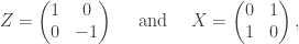
as well as $Y = iZX$ and the identity matrix $I$ , are 1-qubit observables with eigenvalues (i.e. measurement outcomes) $\pm 1$ . Now, take a system of 2 qubits. Since each of the 2 qubits can be either excited or not, our quantum state is a 4-dimensional vector

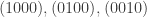
Therein, the 4 vectors $|x\rangle \otimes |y\rangle$ can be identified with the vectors of the canonical basis $(1000), (0100), (0010)$ and $(0001)$ . We will consider the measurement of 2-qubit observables of the form $A \otimes B$ defined by $A \otimes B |x\rangle \otimes |y\rangle = A |x\rangle \otimes B |y\rangle$ . In other words, $A$ acts on the first qubit and $B$ acts on the second one. Later, we will look into the observables $X \otimes I$ , $Z \otimes I$ , $I \otimes X$ , $I \otimes Z$ and their products.

What happens when two observables are measured simultaneously? In quantum mechanics, we can measure simultaneously multiple observables if these observables commute with each other. In that case, measuring $O$ then $O'$ , or measuring $O'$ first and then $O$ , doesn’t make any difference. Therefore, we say that these observables are measured simultaneously, the outcome being a pair $(\lambda,\lambda')$ , composed of an eigenvalue of $O$ and an eigenvalue of $O'$ . Their product $O'' = OO'$ , which commutes with both $O$ and $O'$ , can also be measured in the same time. Measuring this triple returns a triple of eigenvalues $(\lambda,\lambda',\lambda'')$ corresponding respectively to $O$ , $O'$ and $O''$ . The relation $O'' = OO'$ imposes the constraint

(1) $\qquad \lambda'' = \lambda \lambda'$

on the outcomes.

Assume that one can describe the result of all quantum measurements with a model such that, for all observables $O$ and for all states $\nu$ of the model, a deterministic outcome $\lambda_\nu(O)$ exists. Here, $\nu$ is our ‘extended’, not necessarily physical, description of the state of the system. When $O$ and $O'$ are commuting, it is reasonable to assume that the relation (1) holds also at the level of the hidden variable model, namely

(2) $\lambda_\nu(OO') = \lambda_\nu(O) \cdot \lambda_\nu(O').$

Such a model is called a non-contextual hidden variable model. Von Neumann proved that no such value $\lambda_\nu$ exists by considering these relations for all pairs $O$ , $O'$ of observables. This shows that quantum mechanics is contextual! Hum… Wait a minute. It seems silly to impose such a constraint for all pairs of observable, including those that cannot be measured simultaneously. This is “Von Neumann’s silly assumption’. Only pairs of commuting observables should be considered.

Peres-Mermin proof of contextuality

One can resurrect Von Neumann’s argument, assuming Eq.(2) only for commuting observables. Peres-Mermin’s square provides an elegant proof of this result. Form a $3 \times 3$ array with these observables. It is constructed in such a way that

(i) The eigenvalues of all the observables in Peres-Mermin’s square are ±1,

(ii) Each row and each column is a triple of commuting observables,

(iii) The last element of each row and each column is the product of the 2 first observables, except in the last column where $Y \otimes Y = -(Z \otimes Z)(X \otimes X)$ .

If a non-contextual hidden variable exists, it associates fixed eigenvalues $a$ , $b$ , $c$ , $d$ (which are either 1 or -1) with the 4 observables $X \otimes I$ , $Z \otimes I$ , $I \otimes X$ , $I \otimes Z$ . Applying Eq.(2) to the first 2 rows and to the first 2 columns, one deduces the values of all the observables of the square, except $Y \otimes Y$ . Finally, what value should be attributed to $Y \otimes Y$ ? By (iii), applying Eq.(2) to the last row, one gets $\lambda_\nu(Y \otimes Y) = abcd$ . However, using the last column, (iii) and Eq.(2) yield the opposite value $\lambda_\nu (Y \otimes Y ) = -abcd$ . This is the expected contradiction, proving that there is no non-contextual value $\lambda_\nu$ . Quantum mechanics is contextual!

We saw that the randomness in quantum measurements cannot be explained in a ‘classical’ way. Besides its fundamental importance, this result also influences quantum technologies. What I really care about is how to construct a quantum computer, or more generally, I would like to understand what kind of quantum device could be superior to its classical counterpart for certain tasks. Such a quantum advantage can only be reached by exploiting the weirdness of quantum mechanics, such as contextuality ^1,^2,^3,^4,⁵. Understanding these weird phenomena is one of the first tasks to accomplish.

Happy Halloween from…the discrete Wigner function?

Posted on October 23, 2016 by Nicole Yunger Halpern

Do you hope to feel a breath of cold air on the back of your neck this Halloween? I’ve felt one literally: I earned my Masters in the icebox called “Ontario,” at the Perimeter Institute for Theoretical Physics. Perimeter’s colloquia¹ take place in an auditorium blacker than a Quentin Tarantino film. Aephraim Steinberg presented a colloquium one air-conditioned May.

Steinberg experiments on ultracold atoms and quantum optics² at the University of Toronto. He introduced an idea that reminds me of biting into an apple whose coating you’d thought consisted of caramel, then tasting blood: a negative (quasi)probability.

Probabilities usually range from zero upward. Consider Shirley Jackson’s short story The Lottery. Villagers in a 20th-century American village prepare slips of paper. The number of slips equals the number of families in the village. One slip bears a black spot. Each family receives a slip. Each family has a probability $p > 0$ of receiving the marked slip. What happens to the family that receives the black spot? Read Jackson’s story—if you can stomach more than a Tarantino film.

Jackson peeled off skin to reveal the offal of human nature. Steinberg’s experiments reveal the offal of Nature. I’d expect humaneness of Jackson’s villagers and nonnegativity of probabilities. But what looks like a probability and smells like a probability might be hiding its odor with Special-Edition Autumn-Harvest Febreeze.

A quantum state resembles a set of classical³ probabilities. Consider a classical system that has too many components for us to track them all. Consider, for example, the cold breath on the back of your neck. The breath consists of air molecules at some temperature $T$ . Suppose we measured the molecules’ positions and momenta. We’d have some probability $p_1$ of finding this particle here with this momentum, that particle there with that momentum, and so on. We’d have a probability $p_2$ of finding this particle there with that momentum, that particle here with this momentum, and so on. These probabilities form the air’s state.

We can tell a similar story about a quantum system. Consider the quantum light prepared in a Toronto lab. The light has properties analogous to position and momentum. We can represent the light’s state with a mathematical object similar to the air’s probability density.⁴ But this probability-like object can sink below zero. We call the object a quasiprobability, denoted by $\mu$ .

If a $\mu$ sinks below zero, the quantum state it represents encodes entanglement. Entanglement is a correlation stronger than any achievable with nonquantum systems. Quantum information scientists use entanglement to teleport information, encrypt messages, and probe the nature of space-time. I usually avoid this cliché, but since Halloween is approaching: Einstein called entanglement “spooky action at a distance.”

Eugene Wigner and others defined quasiprobabilities shortly before Shirley Jackson wrote The Lottery. Quantum opticians use these $\mu$ ’s, because quantum optics and quasiprobabilities involve continuous variables. Examples of continuous variables include position: An air molecule can sit at this point (e.g., $x = 0$ ) or at that point (e.g., $x = 1$ ) or anywhere between the two (e.g., $x = 0.001$ ). The possible positions form a continuous set. Continuous variables model quantum optics as they model air molecules’ positions.

Information scientists use continuous variables less than we use discrete variables. A discrete variable assumes one of just a few possible values, such as $0$ or $1$ , or trick or treat.

How a quantum-information theorist views Halloween.

Quantum-information scientists study discrete systems, such as electron spins. Can we represent discrete quantum systems with quasiprobabilities $\mu$ as we represent continuous quantum systems? You bet your barmbrack.

Bill Wootters and others have designed quasiprobabilities for discrete systems. Wootters stipulated that his $\mu$ have certain properties. The properties appear in this review. Most physicists label properties “1,” “2,” etc. or “Prop. 1,” “Prop. 2,” etc. The Wootters properties in this review have labels suited to Halloween.

Seeing (quasi)probabilities sink below zero feels like biting into an apple that you think has a caramel coating, then tasting blood. Did you eat caramel apples around age six? Caramel apples dislodge baby teeth. When baby teeth fall out, so does blood. Tasting blood can mark growth—as does the squeamishness induced by a colloquium that spooks a student. Who needs haunted mansions when you have negative quasiprobabilities?

For nonexperts:

¹Weekly research presentations attended by a department.

²Light.

³Nonquantum (basically).

⁴Think “set of probabilities.”

Tripping over my own inner product

Posted on September 18, 2016 by Nicole Yunger Halpern

A scrape stood out on the back of my left hand. The scrape had turned greenish-purple, I noticed while opening the lecture-hall door. I’d jounced the hand against my dining-room table while standing up after breakfast. The table’s corners form ninety-degree angles. The backs of hands do not.

Earlier, when presenting a seminar, I’d forgotten to reference papers by colleagues. Earlier, I’d offended an old friend without knowing how. Some people put their feet in their mouths. I felt liable to swallow a clog.

The lecture was for Ph 219: Quantum Computation. I was TAing (working as a teaching assistant for) the course. John Preskill was discussing quantum error correction.

Computers suffer from errors as humans do: Imagine setting a hard drive on a table. Coffee might spill on the table (as it probably would have if I’d been holding a mug near the table that week). If the table is in my California dining room, an earthquake might judder the table. Juddering bangs the hard drive against the wood, breaking molecular bonds and deforming the hardware. The information stored in computers degrades.

How can we protect information? By encoding it—by translating the message into a longer, encrypted message. An earthquake might judder the encoded message. We can reverse some of the damage by error-correcting.

Different types of math describe different codes. John introduced a type of math called symplectic vector spaces. “Symplectic vector space” sounds to me like a garden of spiny cacti (on which I’d probably have pricked fingers that week). Symplectic vector spaces help us translate between the original and encoded messages.

Symplectic vector space?

Say that an earthquake has juddered our hard drive. We want to assess how the earthquake corrupted the encoded message and to error-correct. Our encryption scheme dictates which operations we should perform. Each possible operation, we represent with a mathematical object called a vector. A vector can take the form of a list of numbers.

We construct the code’s vectors like so. Say that our quantum hard drive consists of seven phosphorus nuclei atop a strip of silicon. Each nucleus has two observables, or measurable properties. Let’s call the observables Z and X.

Suppose that we should measure the first nucleus’s Z. The first number in our symplectic vector is 1. If we shouldn’t measure the first nucleus’s Z, the first number is 0. If we should measure the second nucleus’s Z, the second number is 1; if not, 0; and so on for the other nuclei. We’ve assembled the first seven numbers in our vector. The final seven numbers dictate which nuclei’s Xs we measure. An example vector looks like this: $( 1, \, 0, \, 1, \, 0, \, 1, \, 0, \, 1 \; | \; 0, \, 0, \, 0, \, 0, \, 0, \, 0, \, 0 )$ .

The vector dictates that we measure four Zs and no Xs.

Symplectic vectors represent the operations we should perform to correct errors.

A vector space is a collection of vectors. Many problems—not only codes—involve vector spaces. Have you used Google Maps? Google illustrates the step that you should take next with an arrow. We can represent that arrow with a vector. A vector, recall, can take the form of a list of numbers. The step’s list of two¹numbers indicates whether you should walk $( \text{Northward or not} \; | \; \text{Westward or not} )$ .

I’d forgotten about my scrape by this point in the lecture. John’s next point wiped even cacti from my mind.

Say you want to know how similar two vectors are. You usually calculate an inner product. A vector v tends to have a large inner product with any vector w that points parallel to v.

Parallel vectors tend to have a large inner product.

The vector v tends to have an inner product of zero with any vector w that points perpendicularly. Such v and w are said to annihilate each other. By the end of a three-hour marathon of a research conversation, we might say that v and w “destroy” each other. v is orthogonal to w.

Two orthogonal vectors, having an inner product of zero, annihilate each other.

You might expect a vector v to have a huge inner product with itself, since v points parallel to v. Quantum-code vectors defy expectations. In a symplectic vector space, John said, “you can be orthogonal to yourself.”

A symplectic vector²can annihilate itself, destroy itself, stand in its own way. A vector can oppose itself, contradict itself, trip over its own feet. I felt like I was tripping over my feet that week. But I’m human. A vector is a mathematical ideal. If a mathematical ideal could be orthogonal to itself, I could allow myself space to err.

Tripping over my own inner product.

Lloyd Alexander wrote one of my favorite books, the children’s novel The Book of Three. The novel features a stout old farmer called Coll. Coll admonishes an apprentice who’s burned his fingers: “See much, study much, suffer much.” We smart while growing smarter.

An ant-sized scar remains on the back of my left hand. The scar has been fading, or so I like to believe. I embed references to colleagues’ work in seminar Powerpoints, so that I don’t forget to cite anyone. I apologized to the friend, and I know about symplectic vector spaces. We all deserve space to err, provided that we correct ourselves. Here’s to standing up more carefully after breakfast.

¹Not that I advocate for limiting each coordinate to one bit in a Google Maps vector. The two-bit assumption simplifies the example.

²Not only symplectic vectors are orthogonal to themselves, John pointed out. Consider a string of bits that contains an even number of ones. Examples include (0, 0, 0, 0, 1, 1). Each such string has a bit-wise inner product, over the field ${\mathbb Z}_2$ , of zero with itself.

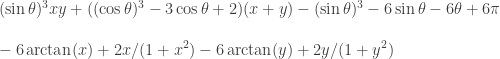
Greg Kuperberg’s calculus problem

Posted on August 3, 2016 by spiros

“How good are you at calculus?”

This was the opening sentence of Greg Kuperberg’s Facebook status on July 4th, 2016.

“I have a joint paper (on isoperimetric inequalities in differential geometry) in which we need to know that

$(\sin\theta)^3 xy + ((\cos\theta)^3 -3\cos\theta +2) (x+y) - (\sin\theta)^3-6\sin\theta -6\theta + 6\pi \\ \\- 6\arctan(x) +2x/(1+x^2) -6\arctan(y) +2y/(1+y^2)$

is non-negative for x and y non-negative and $\theta$ between $0$ and $\pi$ . Also, the minimum only occurs for $x=y=1/(\tan(\theta/2)$ .”

Let’s take a moment to appreciate the complexity of the mathematical statement above. It is a non-linear inequality in three variables, mixing trigonometry with algebra and throwing in some arc-tangents for good measure. Greg, continued:

“We proved it, but only with the aid of symbolic algebra to factor an algebraic variety into irreducible components. The human part of our proof is also not really a cake walk.

A simpler proof would be way cool.”

I was hooked. The cubic terms looked a little intimidating, but if I converted x and y into $\tan(\theta_x)$ and $\tan(\theta_y)$ , respectively, as one of the comments on Facebook promptly suggested, I could at least get rid of the annoying arc-tangents and then calculus and trigonometry would take me the rest of the way. Greg replied to my initial comment outlining a quick route to the proof: “Let me just caution that we found the problem unyielding.” Hmm… Then, Greg revealed that the paper containing the original proof was over three years old (had he been thinking about this since then? that’s what true love must be like.) Titled “The Cartan-Hadamard Conjecture and The Little Prince“, the above inequality makes its appearance as Lemma 7.1 on page 45 (of 63). To quote the paper: “Although the lemma is evident from contour plots, the authors found it surprisingly tricky to prove rigorously.”

As I filled pages of calculations and memorized every trigonometric identity known to man, I realized that Greg was right: the problem was highly intractable. The quick solution that was supposed to take me two to three days turned into two weeks of hell, until I decided to drop the original approach and stick to doing calculus with the known unknowns, x and y. The next week led me to a set of three non-linear equations mixing trigonometric functions with fourth powers of x and y, at which point I thought of giving up. I knew what I needed to do to finish the proof, but it looked freaking insane. Still, like the masochist that I am, I continued calculating away until my brain was mush. And then, yesterday, during a moment of clarity, I decided to go back to one of the three equations and rewrite it in a different way. That is when I noticed the error. I had solved for $\cos\theta$ in terms of x and y, but I had made a mistake that had cost me 10 days of intense work with no end in sight. Once I found the mistake, the whole proof came together within about an hour. At that moment, I felt a mix of happiness (duh), but also sadness, as if someone I had grown fond of no longer had a reason to spend time with me and, at the same time, I had ran out of made-up reasons to hang out with them. But, yeah, I mostly felt happiness.

Greg Kuperberg pondering about the universe of mathematics.

Before I present the proof below, I want to take a moment to say a few words about Greg, whom I consider to be the John Preskill of mathematics: a lodestar of sanity in a sea of hyperbole (to paraphrase Scott Aaronson). When I started grad school at UC Davis back in 2003, quantum information theory and quantum computing were becoming “a thing” among some of the top universities around the US. So, I went to several of the mathematics faculty in the department asking if there was a course on quantum information theory I could take. The answer was to “read Nielsen and Chuang and then go talk to Professor Kuperberg”. Being a foolish young man, I skipped the first part and went straight to Greg to ask him to teach me (and four other brave souls) quantum “stuff”. Greg obliged with a course on… quantum probability and quantum groups. Not what I had in mind. This guy was hardcore. Needless to say, the five brave souls taking the class (mostly fourth year graduate students and me, the noob) quickly became three, then two gluttons for punishment (the other masochist became one of my best friends in grad school). I could not drop the class, not because I had asked Greg to do this as a favor to me, but because I knew that I was in the presence of greatness (or maybe it was Stockholm syndrome). My goal then, as an aspiring mathematician, became to one day have a conversation with Greg where, for some brief moment, I would not sound stupid. A man of incredible intelligence, Greg is that rare individual whose character matches his intellect. Much like the anti-heroes portrayed by Humphrey Bogart in Casablanca and the Maltese Falcon, Greg keeps a low-profile, seems almost cynical at times, but in the end, he works harder than everyone else to help those in need. For example, on MathOverflow, a question and answer website for professional mathematicians around the world, Greg is listed as one of the top contributors of all time.

But, back to the problem. The past four weeks thinking about it have oscillated between phases of “this is the most fun I’ve had in years!” to “this is Greg’s way of telling me I should drop math and become a go-go dancer”. Now that the ordeal is over, I can confidently say that the problem is anything but “dull” (which is how Greg felt others on MathOverflow would perceive it, so he never posted it there). In fact, if I ever have to teach Calculus, I will subject my students to the step-by-step proof of this problem. OK, here is the proof. This one is for you Greg. Thanks for being such a great role model. Sorry I didn’t get to tell you until now. And you are right not to offer a “bounty” for the solution. The journey (more like, a trip to Mordor and back) was all the money.

The proof: The first thing to note (and if I had read Greg’s paper earlier than today, I would have known as much weeks ago) is that the following equality holds (which can be verified quickly by differentiating both sides):

$4 x - 6\arctan(x) +2x/(1+x^2) = 4 \int_0^x \frac{s^4}{(1+s^2)^2} ds$ .

Using the above equality (and the equivalent one for y), we get:

$F(\theta,x,y) = (\sin\theta)^3 xy + ((\cos\theta)^3 -3\cos\theta -2) (x+y) - (\sin\theta)^3-6\sin\theta -6\theta + 6\pi \\ \\4 \int_0^x \frac{s^4}{(1+s^2)^2} ds+4 \int_0^y \frac{s^4}{(1+s^2)^2} ds.$

Now comes the fun part. We differentiate with respect to $\theta$ , x and y, and set to zero to find all the maxima and minima of $F(\theta,x,y)$ (though we are only interested in the global minimum, which is supposed to be at $x=y=\tan^{-1}(\theta/2))$ . Some high-school level calculus yields:

$\partial_\theta F(\theta,x,y) = 0 \implies \sin^2(\theta) (\cos(\theta) xy + \sin(\theta)(x+y)) = \\ \\ 2 (1+\cos(\theta))+\sin^2(\theta)\cos(\theta).$

At this point, the most well-known trigonometric identity of all time, $\sin^2(\theta)+\cos^2(\theta)=1$ , can be used to show that the right-hand-side can be re-written as:

$2(1+\cos(\theta))+\sin^2(\theta)\cos(\theta) = \sin^2(\theta) (\cos\theta \tan^{-2}(\theta/2) + 2\sin\theta \tan^{-1}(\theta/2)),$

where I used (my now favorite) trigonometric identity: $\tan^{-1}(\theta/2) = (1+\cos\theta)/\sin(\theta)$ (note to the reader: $\tan^{-1}(\theta) = \cot(\theta)$ ). Putting it all together, we now have the very suggestive condition:

$\sin^2(\theta) (\cos(\theta) (xy-\tan^{-2}(\theta/2)) + \sin(\theta)(x+y-2\tan^{-1}(\theta/2))) = 0,$

noting that, despite appearances, $\theta = 0$ is not a solution (as can be checked from the original form of this equality, unless $x$ and $y$ are infinite, in which case the expression is clearly non-negative, as we show towards the end of this post). This leaves us with $\theta = \pi$ and

$\cos(\theta) (\tan^{-2}(\theta/2)-xy) = \sin(\theta)(x+y-2\tan^{-1}(\theta/2)),$

as candidates for where the minimum may be. A quick check shows that:

$F(\pi,x,y) = 4 \int_0^x \frac{s^4}{(1+s^2)^2} ds+4 \int_0^y \frac{s^4}{(1+s^2)^2} ds \ge 0,$

since x and y are non-negative. The following obvious substitution becomes our greatest ally for the rest of the proof:

$x= \alpha \tan^{-1}(\theta/2), \, y = \beta \tan^{-1}(\theta/2).$

Substituting the above in the remaining condition for $\partial_\theta F(\theta,x,y) = 0$ , and using again that $\tan^{-1}(\theta/2) = (1+\cos\theta)/\sin\theta$ , we get:

$\cos\theta (1-\alpha\beta) = (1-\cos\theta) ((\alpha-1) + (\beta-1)),$

which can be further simplified to (if you are paying attention to minus signs and don’t waste a week on a wild-goose chase like I did):

$\cos\theta = \frac{1}{1-\beta}+\frac{1}{1-\alpha}$ .

As Greg loves to say, we are finally cooking with gas. Note that the expression is symmetric in $\alpha$ and $\beta$ , which should be obvious from the symmetry of $F(\theta,x,y)$ in x and y. That observation will come in handy when we take derivatives with respect to x and y now. Factoring $(\cos\theta)^3 -3\cos\theta -2 = - (1+\cos\theta)^2(2-\cos\theta)$ , we get:

$\partial_x F(\theta,x,y) = 0 \implies \sin^3(\theta) y + 4\frac{x^4}{(1+x^2)^2} = (1+\cos\theta)^2 + \sin^2\theta (1+\cos\theta).$

Substituting x and y with $\alpha \tan^{-1}(\theta/2), \beta \tan^{-1}(\theta/2)$ , respectively and using the identities $\tan^{-1}(\theta/2) = (1+\cos\theta)/\sin\theta$ and $\tan^{-2}(\theta/2) = (1+\cos\theta)/(1-\cos\theta),$ the above expression simplifies significantly to the following expression:

$4\alpha^4 =\left((\alpha^2-1)\cos\theta+\alpha^2+1\right)^2 \left(1 + (1-\beta)(1-\cos\theta)\right).$

Using $\cos\theta = \frac{1}{1-\beta}+\frac{1}{1-\alpha}$ , which we derived earlier by looking at the extrema of $F(\theta,x,y)$ with respect to $\theta$ , and noting that the global minimum would have to be an extremum with respect to all three variables, we get:

$4\alpha^4 (1-\beta) = \alpha (\alpha-1) (1+\alpha + \alpha(1-\beta))^2,$

where we used $1 + (1-\beta)(1-\cos\theta) = \alpha (1-\beta) (\alpha-1)^{-1}$ and

$(\alpha^2-1)\cos\theta+\alpha^2+1 = (\alpha+1)((\alpha-1)\cos\theta+1)+\alpha(\alpha-1) = \\ (\alpha-1)(1-\beta)^{-1} (2\alpha + 1-\alpha\beta).$

We may assume, without loss of generality, that $x \ge y$ . If $\alpha = 0$ , then $\alpha = \beta = 0$ , which leads to the contradiction $\cos\theta = 2$ , unless the other condition, $\theta = \pi$ , holds, which leads to $F(\pi,0,0) = 0$ . Dividing through by $\alpha$ and re-writing $4\alpha^3(1-\beta) = 4\alpha(1+\alpha)(\alpha-1)(1-\beta) + 4\alpha(1-\beta)$ , yields:

$4\alpha (1-\beta) = (\alpha-1) (1+\alpha - \alpha(1-\beta))^2 = (\alpha-1)(1+\alpha\beta)^2,$

which can be further modified to:

$4\alpha +(1-\alpha\beta)^2 = \alpha (1+\alpha\beta)^2,$

and, similarly for $\beta$ (due to symmetry):

$4\beta +(1-\alpha\beta)^2 = \beta (1+\alpha\beta)^2.$

Subtracting the two equations from each other, we get:

$4(\alpha-\beta) = (\alpha-\beta)(1+\alpha\beta)^2$ ,

which implies that $\alpha = \beta$ and/or $\alpha\beta =1$ . The first leads to $4\alpha (1-\alpha) = (\alpha-1)(1+\alpha^2)^2,$ which immediately implies $\alpha = 1 = \beta$ (since the left and right side of the equality have opposite signs otherwise). The second one implies that either $\alpha+\beta =2$ , or $\cos\theta =1$ , which follows from the earlier equation $\cos\theta (1-\alpha\beta) = (1-\cos\theta) ((\alpha-1) + (\beta-1))$ . If $\alpha+\beta =2$ and $1 = \alpha\beta$ , it is easy to see that $\alpha=\beta=1$ is the only solution by expanding $(\sqrt{\alpha}-\sqrt{\beta})^2=0$ . If, on the other hand, $\cos\theta = 1$ , then looking at the original form of $F(\theta,x,y)$ , we see that $F(0,x,y) = 6\pi - 6\arctan(x) +2x/(1+x^2) -6\arctan(y) +2y/(1+y^2) \ge 0$ , since $x,y \ge 0 \implies \arctan(x)+\arctan(y) \le \pi$ .

And that concludes the proof, since the only cases for which all three conditions are met lead to $\alpha = \beta = 1$ and, hence, $x=y=\tan^{-1}(\theta/2)$ . The minimum of $F(\theta, x,y)$ at these values is always zero. That’s right, all this work to end up with “nothing”. But, at least, the last four weeks have been anything but dull.

Update: Greg offered Lemma 7.4 from the same paper as another challenge (the sines, cosines and tangents are now transformed into hyperbolic trigonometric functions, with a few other changes, mostly in signs, thrown in there). This is a more hardcore-looking inequality, but the proof turns out to follow the steps of Lemma 7.1 almost identically. In particular, all the conditions for extrema are exactly the same, with the only difference being that cosine becomes hyperbolic cosine. It is an awesome exercise in calculus to check this for yourself. Do it. Unless you have something better to do.

Bringing the heat to Cal State LA

Posted on July 24, 2016 by Nicole Yunger Halpern

John Baez is a tough act to follow.

The mathematical physicist presented a colloquium at Cal State LA this May.¹ The talk’s title: “My Favorite Number.” The advertisement image: A purple “24” superimposed atop two egg cartons.

The colloquium concerned string theory. String theorists attempt to reconcile Einstein’s general relativity with quantum mechanics. Relativity concerns the large and the fast, like the sun and light. Quantum mechanics concerns the small, like atoms. Relativity and with quantum mechanics individually suggest that space-time consists of four dimensions: up-down, left-right, forward-backward, and time. String theory suggests that space-time has more than four dimensions. Counting dimensions leads theorists to John Baez’s favorite number.

His topic struck me as bold, simple, and deep. As an otherworldly window onto the pedestrian. John Baez became, when I saw the colloquium ad, a hero of mine.

And a tough act to follow.

I presented Cal State LA’s physics colloquium the week after John Baez. My title: “Quantum steampunk: Quantum information applied to thermodynamics.” Steampunk is a literary, artistic, and film genre. Stories take place during the 1800s—the Victorian era; the Industrial era; an age of soot, grime, innovation, and adventure. Into the 1800s, steampunkers transplant modern and beyond-modern technologies: automata, airships, time machines, etc. Example steampunk works include Will Smith’s 1999 film Wild Wild West. Steampunk weds the new with the old.

So does quantum information applied to thermodynamics. Thermodynamics budded off from the Industrial Revolution: The steam engine crowned industrial technology. Thinkers wondered how efficiently engines could run. Thinkers continue to wonder. But the steam engine no longer crowns technology; quantum physics (with other discoveries) does. Quantum information scientists study the roles of information, measurement, and correlations in heat, energy, entropy, and time. We wed the new with the old.

What image could encapsulate my talk? I couldn’t lean on egg cartons. I proposed a steampunk warrior—cravatted, begoggled, and spouting electricity. The proposal met with a polite cough of an email. Not all department members, Milan Mijic pointed out, had heard of steampunk.

Milan is a Cal State LA professor and my erstwhile host. We toured the palm-speckled campus around colloquium time. What, he asked, can quantum information contribute to thermodynamics?

Heat offers an example. Imagine a classical (nonquantum) system of particles. The particles carry kinetic energy, or energy of motion: They jiggle. Particles that bump into each other can exchange energy. We call that energy heat. Heat vexes engineers, breaking transistors and lowering engines’ efficiencies.

Like heat, work consists of energy. Work has more “orderliness” than the heat transferred by random jiggles. Examples of work exertion include the compression of a gas: A piston forces the particles to move in one direction, in concert. Consider, as another example, driving electrons around a circuit with an electric field. The field forces the electrons to move in the same direction. Work and heat account for all the changes in a system’s energy. So states the First Law of Thermodynamics.

Suppose that the system is quantum. It doesn’t necessarily have a well-defined energy. But we can stick the system in an electric field, and the system can exchange motional-type energy with other systems. How should we define “work” and “heat”?

Quantum information offers insights, such as via entropies. Entropies quantify how “mixed” or “disordered” states are. Disorder grows as heat suffuses a system. Entropies help us extend the First Law to quantum theory.

So I explained during the colloquium. Rarely have I relished engaging with an audience as much as I relished engaging with Cal State LA’s. Attendees made eye contact, posed questions, commented after the talk, and wrote notes. A student in a corner appeared to be writing homework solutions. But a presenter couldn’t have asked for more from the rest. One exclamation arrested me like a coin in the cogs of a grandfather clock.

I’d peppered my slides with steampunk art: paintings, drawings, stills from movies. The peppering had staved off boredom as I’d created the talk. I hoped that the peppering would stave off my audience’s boredom. I apologized about the trimmings.

“No!” cried a woman near the front. “It’s lovely!”

I was about to discuss experiments by Jukka Pekola’s group. Pekola’s group probes quantum thermodynamics using electronic circuits. The group measures heat by counting the electrons that hop from one part of the circuit to another. Single-electron transistors track tunneling (quantum movements) of single particles.

Heat complicates engineering, calculations, and California living. Heat scrambles signals, breaks devices, and lowers efficiencies. Quantum heat can evade definition. Thermodynamicists grind their teeth over heat.

“No!” the woman near the front had cried. “It’s lovely!”

She was referring to steampunk art. But her exclamation applied to my subject. Heat has not only practical importance, but also fundamental: Heat influences every law of thermodynamics. Thermodynamic law underpins much of physics as 24 underpins much of string theory. Lovely, I thought, indeed.

Cal State LA offered a new view of my subfield, an otherworldly window onto the pedestrian. The more pedestrian an idea—the more often the idea surfaces, the more of our world the idea accounts for—the deeper the physics. Heat seems as pedestrian as a Pokémon Go player. But maybe, someday, I’ll present an idea as simple, bold, and deep as the number 24.

A window onto Cal State LA.

With gratitude to Milan Mijic, and to Cal State LA’s Department of Physics and Astronomy, for their hospitality.

¹For nonacademics: A typical physics department hosts several presentations per week. A seminar relates research that the speaker has undertaken. The audience consists of department members who specialize in the speaker’s subfield. A department’s astrophysicists might host a Monday seminar; its quantum theorists, a Wednesday seminar; etc. One colloquium happens per week. Listeners gather from across the department. The speaker introduces a subfield, like the correction of errors made by quantum computers. Course lectures target students. Endowed lectures, often named after donors, target researchers.

Quantum Frontiers

A blog by the Institute for Quantum Information and Matter @ Caltech

Category Archives: Theoretical highlights

Here’s one way to get out of a black hole!

Local operations and Chinese communications

It’s CHAOS!

Hamiltonian: An American Musical (without Americana or music)

The weak shall inherit the quasiprobability.

Good news everyone! Flatland is non-contextual!

Happy Halloween from…the discrete Wigner function?

Tripping over my own inner product

Greg Kuperberg’s calculus problem

Bringing the heat to Cal State LA

Share this:

Share this:

Share this:

Share this:

Share this:

Share this:

Share this:

Share this:

Share this:

Share this: